小果又来分享啦!今天小果为小伙伴带来的分享为利用quanTIseq算法进行免疫浸润分析,然后基于亚型分组信息文件,进行亚型间免疫细胞含量显著差异分析,该分析在肿瘤生信文章中必备的分析内容,非常值得小伙伴学习,小果强烈推荐呀!接下来跟着小果开启开始今天的分享学习。
- quanTIseq算法介绍
在进行该分析之前,小果先简单介绍一下quanTIseq算法,quanTIseq基于反卷积算法,利用bulk samples的RNA_seq数据,可以对肿瘤样本中不同种类免疫细胞的组成进行预测,支持10种类型的免疫细胞,包括B cells,Classically activated macrophages (M1),Alternatively activated macrophages (M2),Monocytes,Neutrophils,Natural killer (NK) cells,Non-regulatory CD4+ T cells ,CD8+ T cells,Dendritic cells,Other uncharacterized cells,这就是小果对该算法的介绍,想深入学习的小伙伴可以到该网址:https://icbi.i-med.ac.at/software/quantiseq/doc/index.html#Figure1。
#首先下载quanTIseq流程分析脚本,如下文:
wget https://icbi.i-med.ac.at/software/quantiseq/doc/downloads/quanTIseq_pipeline.sh
#quanTIseq流程运行参数使用方法

- 准备需要的R包
#安装需要的包
install.packages(“ggplot2”)
install.packages(“ggsci”)
install.packages(“tidyverse”)
install.packages(“reshape2”)
install.packages(“ggpubr”)
#加载需要的R包
library(reshape2)
library(ggpubr)
library(ggplot2)
library(tidyverse)
library(ggsci)
2.输入数据
#EXP.txt,基因表达矩阵文件,行名为基因名,列名为样本信息。
exp<-read.table(“EXP.txt”,header=T,row.names=1,sep=”\t”,check.names=F)

#将行名转化为列名
exp<-rownames_to_column(exp,var=”GENE”)
4.利用quanTIseq算法进行免疫浸润分析
#quanTIseq进行免疫浸润分析
bash quanTIseq_pipeline.sh –inputfile=exp.txt –outputdir=quanTIseqTest –prefix=quanTIseqTest –pipelinestart=decon
input表示基因表达矩阵,第一列为基因名,其他列为样本名。
outputdir表示生成结果文件名
prefix表示生成结果文件前缀
pipelinestart表示quanTIseq分析流程,基因表达矩阵选用decon
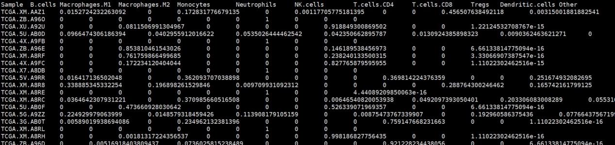
#生成结果文件为quanTIseqTest_cell_fractions.txt,该结果为计算的10种免疫细胞在不同样本中的含量,第一列为样本名,其他列为免疫细胞类型。
5.不同亚型中quanTIseq算法计算的免疫细胞的显著差异分析
#读取quanTIseq分析免疫细胞组成结果文件
immune<-read.table(“quanTIseqTest_cell_fractions.txt”,header=T,sep=”\t”)
#将Sample列”.”修改为”-”
immune$Sample<-str_replace_all(immune$Sample,”\\.”,”-“)
#亚型分组文件,行名为样本信息,第一列为样本信息,第二列为亚型分组信息。
K3<-read.table(“K3.txt”,header=T,sep=”\t”)

#合并免疫细胞组成文件和亚型分组文件
final<-left_join(immune,K3,by=”Sample”)
#长宽数据转换
quanTIseq_cluster<-melt(final,id.vars=c(“Sample”,”Cluster”))
#设置列名
colnames(quanTIseq_cluster)<-c(“Sample”,”Cluster”,”celltype”,”quanTIseq”)
#绘制显著差异分析小提琴+箱线图
boxplot_quanTIseq<- ggplot(quanTIseq_cluster, aes(x = celltype, y =quanTIseq ))+
labs(y=”quanTIseq”,x= “”)+
geom_boxplot(aes(fill = Cluster),position=position_dodge(0.5),width=0.5)+
scale_fill_npg()+
#修改主题
theme_classic() +
theme(axis.title = element_text(size = 12,color =”black”),
axis.text = element_text(size= 12,color = “black”),
panel.grid.minor.y = element_blank(),
panel.grid.minor.x = element_blank(),
axis.text.x = element_text(angle = 45, hjust = 1 ),
panel.grid=element_blank(),
legend.position = “top”,
legend.text = element_text(size= 12),
legend.title= element_text(size= 12)
) +
stat_compare_means(aes(group = Cluster),
label = “p.signif”,
method = “kruskal.test”,#kruskal.test多组检验
hide.ns = F)#隐藏不显著的
#保存图片
ggsave(file=”quanTIseq.pdf”,boxplot_quanTIseq,height=10,width=15)

最终小果成功的对不同亚型利用quanTIseq算法进行了免疫浸润分析,,看起来图片效果非常不错,欢迎大家和小果一起讨论学习呀!免疫浸润相关分析内容,例如单样本富集算法分析免疫浸润丰度(http://www.biocloudservice.com/106/106.php),计算64种免疫细胞相对含量(http://www.biocloudservice.com/107/107.php),panImmune免疫浸润分析(http://www.biocloudservice.com/782/782.php)等都可以用本公司新开发的零代码云平台生信分析小工具,一键完成该分析奥,感兴趣的小伙伴欢迎来尝试奥,网址:http://www.biocloudservice.com/home.html。今天小果的分享就到这里,下期在见奥。
生信小白的福利,利用quanTIseq算法进行免疫浸润分析
小果又来分享啦!今天小果为小伙伴带来的分享为利用quanTIseq算法进行免疫浸润分析,然后基于亚型分组信息文件,进行亚型间免疫细胞含量显著差异分析,该分析在肿瘤生信文章中必备的分析内容,非常值得小伙伴学习,小果强烈推荐呀!接下来跟着小果开启开始今天的分享学习。
- quanTIseq算法介绍
在进行该分析之前,小果先简单介绍一下quanTIseq算法,quanTIseq基于反卷积算法,利用bulk samples的RNA_seq数据,可以对肿瘤样本中不同种类免疫细胞的组成进行预测,支持10种类型的免疫细胞,包括B cells,Classically activated macrophages (M1),Alternatively activated macrophages (M2),Monocytes,Neutrophils,Natural killer (NK) cells,Non-regulatory CD4+ T cells ,CD8+ T cells,Dendritic cells,Other uncharacterized cells,这就是小果对该算法的介绍,想深入学习的小伙伴可以到该网址:https://icbi.i-med.ac.at/software/quantiseq/doc/index.html#Figure1。
#首先下载quanTIseq流程分析脚本,如下文:
wget https://icbi.i-med.ac.at/software/quantiseq/doc/downloads/quanTIseq_pipeline.sh
#quanTIseq流程运行参数使用方法
- 准备需要的R包
#安装需要的包
install.packages(“ggplot2”)
install.packages(“ggsci”)
install.packages(“tidyverse”)
install.packages(“reshape2”)
install.packages(“ggpubr”)
#加载需要的R包
library(reshape2)
library(ggpubr)
library(ggplot2)
library(tidyverse)
library(ggsci)
2.输入数据
#EXP.txt,基因表达矩阵文件,行名为基因名,列名为样本信息。
exp<-read.table(“EXP.txt”,header=T,row.names=1,sep=”\t”,check.names=F)
#将行名转化为列名
exp<-rownames_to_column(exp,var=”GENE”)
4.利用quanTIseq算法进行免疫浸润分析
#quanTIseq进行免疫浸润分析
bash quanTIseq_pipeline.sh –inputfile=exp.txt –outputdir=quanTIseqTest –prefix=quanTIseqTest –pipelinestart=decon
input表示基因表达矩阵,第一列为基因名,其他列为样本名。
outputdir表示生成结果文件名
prefix表示生成结果文件前缀
pipelinestart表示quanTIseq分析流程,基因表达矩阵选用decon
#生成结果文件为quanTIseqTest_cell_fractions.txt,该结果为计算的10种免疫细胞在不同样本中的含量,第一列为样本名,其他列为免疫细胞类型。
5.不同亚型中quanTIseq算法计算的免疫细胞的显著差异分析
#读取quanTIseq分析免疫细胞组成结果文件
immune<-read.table(“quanTIseqTest_cell_fractions.txt”,header=T,sep=”\t”)
#将Sample列”.”修改为”-”
immune$Sample<-str_replace_all(immune$Sample,”\\.”,”-“)
#亚型分组文件,行名为样本信息,第一列为样本信息,第二列为亚型分组信息。
K3<-read.table(“K3.txt”,header=T,sep=”\t”)
#合并免疫细胞组成文件和亚型分组文件
final<-left_join(immune,K3,by=”Sample”)
#长宽数据转换
quanTIseq_cluster<-melt(final,id.vars=c(“Sample”,”Cluster”))
#设置列名
colnames(quanTIseq_cluster)<-c(“Sample”,”Cluster”,”celltype”,”quanTIseq”)
#绘制显著差异分析小提琴+箱线图
boxplot_quanTIseq<- ggplot(quanTIseq_cluster, aes(x = celltype, y =quanTIseq ))+
labs(y=”quanTIseq”,x= “”)+
geom_boxplot(aes(fill = Cluster),position=position_dodge(0.5),width=0.5)+
scale_fill_npg()+
#修改主题
theme_classic() +
theme(axis.title = element_text(size = 12,color =”black”),
axis.text = element_text(size= 12,color = “black”),
panel.grid.minor.y = element_blank(),
panel.grid.minor.x = element_blank(),
axis.text.x = element_text(angle = 45, hjust = 1 ),
panel.grid=element_blank(),
legend.position = “top”,
legend.text = element_text(size= 12),
legend.title= element_text(size= 12)
) +
stat_compare_means(aes(group = Cluster),
label = “p.signif”,
method = “kruskal.test”,#kruskal.test多组检验
hide.ns = F)#隐藏不显著的
#保存图片
ggsave(file=”quanTIseq.pdf”,boxplot_quanTIseq,height=10,width=15)
最终小果成功的对不同亚型利用quanTIseq算法进行了免疫浸润分析,,看起来图片效果非常不错,欢迎大家和小果一起讨论学习呀!免疫浸润相关分析内容,例如单样本富集算法分析免疫浸润丰度(http://www.biocloudservice.com/106/106.php),计算64种免疫细胞相对含量(http://www.biocloudservice.com/107/107.php),panImmune免疫浸润分析(http://www.biocloudservice.com/782/782.php)等都可以用本公司新开发的零代码云平台生信分析小工具,一键完成该分析奥,感兴趣的小伙伴欢迎来尝试奥,网址:http://www.biocloudservice.com/home.html。今天小果的分享就到这里,下期在见奥。