在精准医学的领域,如何确定药物强大的生物标志物是研究人员一直面临的一个巨大挑战,虽然患者源性肿瘤异种移植(PDX)已经是非常可靠的临床前模型了,但是缺乏计算工具使得分析PDX的高通量分子和药理学特征变得特别困难,因此,小果今天给大家介绍的就是精准医学关键挑战的破局者——Xeva。
Xeva (XEnograft Visualization & Analysis),是一个用于体内药物基因组学数据集的开源软件包, 可以量化基因表达的可变性和跨PDX传代的途径活性。
Xeva通过使用迄今为止最大的PDX药物基因组数据集,确定了87种与51种药物反应显著相关的途径(FDR<0.05)。发现了基于基因表达、拷贝数畸变和突变预测药物反应的新的生物标志物(一致性指数>0.60;FDR< 0.05)。总之,Xeva为临床前体内药物基因组学数据的综合分析提供了一个灵活的平台,以识别预测药物反应的生物标志物,代表着精准肿瘤学的重要一步!
介绍了这么多,小果已经跃跃欲试啦!今天小果就来手把手教会大家如何使用Xeva这个R包。本次教程对电脑配置有一定需求,建议大家使用服务器运行,如果没有自己的服务器,欢迎联系我们来租赁服务器哦~
Step 1 安装Xeva
分析所需的数据小果已经帮大家准备好了~
链接:https://pan.baidu.com/s/1E9LxoIqMYYvBJKtkSkGN4A
提取码:x54w
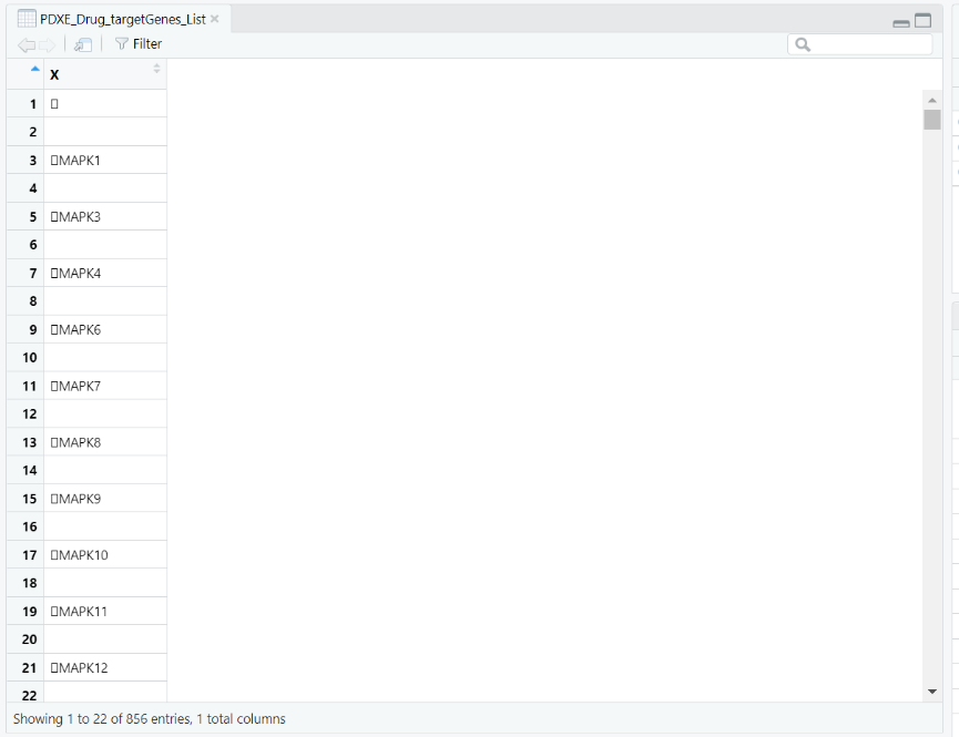
图中的数据是我们本次分析所涉及到的一些药物通路,例如图中给出了MAPK相关的信号通路。
#检查和安装Xeva
library(devtools)
if(is.element(“Xeva”, installed.packages())==FALSE)
{
install_github(“bhklab/Xeva”)
}
library(Xeva)
Step 2 分析药物对于乳腺癌的有效性
#安装所需R包
library(methods)
library(BBmisc)
library(Xeva)
#加载患者的肿瘤反应数据
data(pdxe)
#将肿瘤的缩写和全称对应,方便绘图
tumor <- c(“BRCA” = “Breast Cancer”,
“NSCLC” = “Non-small Cell Lung Carcinoma”,
“PDAC” = “Pancreatic Ductal Carcinoma”,
“CM” = “Cutaneous Melanoma”,
“GC” = “Gastric Cancer”,
“CRC” = “Colorectal Cancer”)
#输出PDF文件,根据Xeva中的mRECIST 标准,按照患者的ID和肿瘤类型进行了分组,得到了一个新的数据集 pdxe.tt
pdf(“../results/figure-1.pdf”, width = 14.1, height = 7.6)
for(tt in names(tumor))
{
pdxe.tt <- summarizeResponse(pdxe, response.measure = “mRECIST”,
group.by=”patient.id”, tissue=tt)
pdxe.tt <- pdxe.tt[, names(sort(pdxe.tt[“untreated”, ], na.last = TRUE))]
plotmRECIST(pdxe.tt, control.name = “Untreated”, name = tumor[tt],
row_fontsize = 12, col_fontsize=12, sort = FALSE)
}
dev.off()
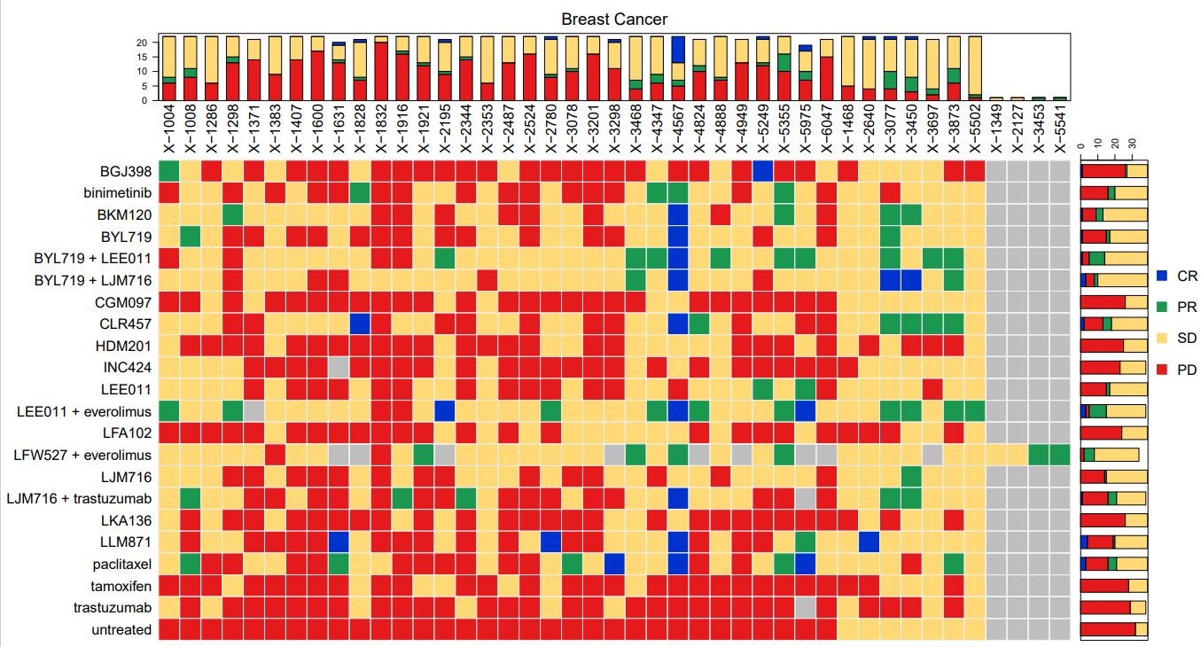
通过使用Xeva的mRECIST函数计算和可视化PDXE乳腺癌数据中基于PDX的药物筛选的响应。
从图片中可以看到,有些治疗的效果比较好,比如 BGJ398 和 binimetinib,有很多红色的格子,表示完全反应(CR)。有些治疗的效果比较差,比如 paclitaxel 和 LLM871,它们有很多蓝色的格子,表示进展性疾病(PD)。有些治疗的效果比较一般,比如LEE011+everolimus,有很多绿色的格子,表示稳定病情(SD)。可以帮助研究人员分析哪些药物对哪些患者有效,以及哪些药物可能有副作用或无效。
Step 3 对基因数据进行TSNE分析,相关性分析
#导入功能函数,所用包
set.seed(19)
#调用功能函数文件
source(“imp_functions.R”)
suppressMessages(library(Biobase))
library(Rtsne)
library(ggplot2)
library(ggpubr)
#准备输出结果
args <- commandArgs(trailingOnly = TRUE)
recompute <- FALSE
if(args[1] %in% c(TRUE, FALSE))
{ recompute <- args[1] }
pdf(“../results/figure-2.pdf”, width = 9.27, height = 6.4)
#从”../data/passage_data.Rda”文件中读取通道数据。
passage <- readRDS(“../data/passage_data.Rda”)
dp <- pData(passage$data)
#对数据进行t-SNE(t分布随机邻居嵌入)降维处理
#计算肿瘤对应的患者数量,排序
ptByTT <- sort(sapply(unique(dp$tumor.type),
function(tt){length(unique(dp[dp$tumor.type==tt, “patient.id”]))},
USE.NAMES = TRUE))
#筛选数量大于10的肿瘤类型
tt2take <- names(ptByTT)[ptByTT>10]
dq <- dp[dp$tumor.type %in% tt2take, ]
psgFrq<- table(dq$patient.id)
pid2take <- names(psgFrq)[psgFrq>1]
dq <- dq[dq$patient.id%in%pid2take, ]
dq$tumor.type <- gsub(“_”, ” “, dq$tumor.type)
dq$tumor.type[dq$tumor.type==”large intestine”] <- “LI”
tissuCol <- c(‘#1b9e77′,’#d95f02′,’#7570b3′,’#e7298a’, ‘#d9f0a3’, ‘#e6ab02′,’#a6761d’,’#666666′)
names(tissuCol) <- c(“lung”, “ovary”, “LI”, “breast”, “kidney”, “pancreas”,
“skin”, “soft tissue”)
#筛选数据
dt <- as.matrix(t(Biobase::exprs(passage$data)))
dt <- dt[dq$biobase.id, ]
#运行t-SNE算法分析
tsne_out <- Rtsne(dt, perplexity = 13)
dq$X <- data.frame(tsne_out$Y)[,1]
dq$Y <- data.frame(tsne_out$Y)[,2]
#进行可视化分析
tsne.plot <- ggplot(data=dq, aes(X, Y, color=tumor.type)) + geom_point(size=0.5)
tsne.plot <- tsne.plot + theme_classic()
tsne.plot <- tsne.plot + scale_color_manual(values=tissuCol)
tsne.plot <- tsne.plot + geom_line(data=dq, aes(X, Y, group=patient.id),
show.legend=FALSE)
print(tsne.plot)
#对肿瘤数据的相关性进行分析
marExp <- Biobase::exprs(passage$data)
passMat <- passage$passage
# 过滤有多个非 NA 值的行和列
passMat <- passMat %>%
filter(rowSums(!is.na(.)) > 1) %>%
filter(colSums(!is.na(.)) > 1)
if(recompute==TRUE)
{
cat(sprintf(“recomputing values…. it may take long time\n”))
dfx <- data.frame()
##—– correlation for related pairs ————
# use map_dfr to loop over the rows and return a data frame
dfx <- passMat %>%
map_dfr(~{
# use combn to get all possible pairs of non-NA values
prx <- combn(.x[!is.na(.x)], 2, simplify = F)
# use map_dbl to loop over the pairs and return a numeric vector
v <- prx %>%
map_dbl(~cor(marExp[, .x[1]], marExp[, .x[2]], method = “pearson”))
# return a data frame with correlation and type
data.frame(Correlation = v, type = “Related pairs”)
})
# 使用 sample_n 获取行的随机样本
randPassMat <- passMat %>%
sample_n(nrow(passMat))
# 使用 map_dfr 遍历行并返回数据帧
dfx <- randPassMat %>%
map_dfr(~{
# use combn to get all possible pairs of non-NA values
prx <- combn(.x[!is.na(.x)], 2, simplify = F)
# use keep to filter the pairs that are not in the same row of passMat
prx <- prx %>%
keep(~!any(passMat[which(passMat == .x[1]), ] == .x[2]))
#使用 map_dbl 遍历这些对并返回一个数值向量
v <- prx %>%
map_dbl(~cor(marExp[, .x[1]], marExp[, .x[2]]))
# return a data frame with correlation and type
data.frame(Correlation = v, type = “Random pairs”)
})
} else
{
cat(sprintf(“using pre-computed values\n”))
dfx <- readRDS(“../data/PDX_passage_correlation.Rda”)
}
pltOrd <- c(“Related pairs”, “Random pairs”)
dfx$type <- factor(as.character(dfx$type), levels = pltOrd)
pltCol <- c(‘#e41a1c’,’#377eb8′)
names(pltCol) <- pltOrd
#创建小提琴图和摘要统计数据,以比较相关对和随机对之间的相关性
p <- ggplot(data=dfx, aes(x=type, y=Correlation, fill=type, color=type))
p <- p + geom_violin(trim=T)
p <- p + theme_classic()
p <- p + scale_fill_manual(values=pltCol)
p <- p + scale_color_manual(values=pltCol)
p <- p + stat_summary(fun.data=data_summary, colour = “white”, size=0.4)
p <- p + theme(legend.position=”none”)
p <- p + scale_y_continuous(breaks = seq(-1,1,by = 0.1))
p <- p + theme(axis.text.x = element_text(colour=”grey20″,size=12, angle=0,face=”bold”),
axis.text.y = element_text(colour=”grey20″,size=11, face=”bold”),
axis.title.y = element_text(colour=”grey20″,size=11, face=”bold”),
axis.ticks.length=unit(0.25,”cm”))
p <- p + theme(axis.line.x = element_line(size = 0, colour = “white”),
axis.title.x=element_blank(),
axis.ticks.x=element_blank())
comparisons <- list(c(“Related pairs”, “Random pairs”))
p <- p + stat_compare_means(comparisons = comparisons, label = “p.signif”)
print(p)
dev.off()
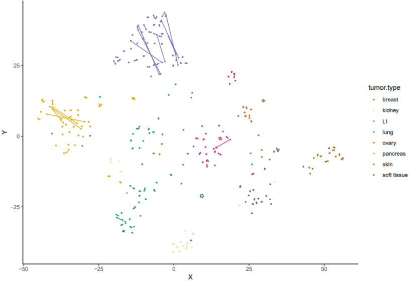
结果如图,左图是对PDXs不同传代17304个基因的基因表达数据进行TSNE分析,从而将高维数据映射到低维空间,显示了不同类型的肿瘤在二维空间中的分布。每种颜色代表一种特定类型的肿瘤,比如说乳腺癌(紫色)的数据点分布得比较广泛,有些点与其他类型的肿瘤混合在一起,有些点则形成了一些簇。这可能表明乳腺癌的异质性比较高,有些亚型与其他类型的肿瘤更相似,有些亚型则更独特。
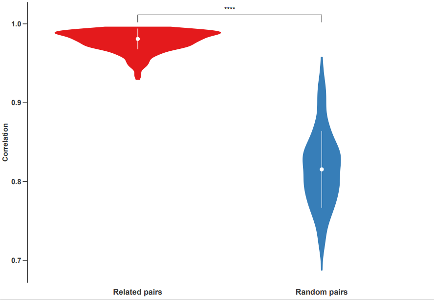
而右图是相关样本对(属于同一谱系)和随机选择样本对的Pearson相关性的可视化,从这幅图中,我们可以看到:相关对的相关性的平均值是0.94,随机对的相关性的平均值是0.86,说明两者之间有显著的差异。
Step 4 所有基因在PDX传代中的类内相关性(ICC)可视化
#导入包
source(“imp_functions.R”)
library(foreach)
library(doParallel)
library(psych)
##plotViolin:使用ggplot2包生成小提琴图。
plotViolin <- function(dfx, pltCol, ylim=NULL)
{
p <- ggplot(data=dfx, aes(x=type, y=ICC , fill=type,color=type))
p <- p + geom_boxplot(width = .001, outlier.size = 2.0, outlier.color = “#525252”,
outlier.shape = 95)
p <- p + geom_violin(trim=F)
p <- p + theme_classic()
p <- p + scale_fill_manual(values=pltCol)
p <- p + scale_color_manual(values=pltCol)
p <- p + stat_summary(fun.data=data_summary, colour = “white”, size=0.4)
p <- p + theme(legend.position=”none”)
p <- p + scale_y_continuous(breaks = seq(-1,1,by = 0.25))
p <- p + theme(axis.text.x = element_text(colour=”grey20″,size=12, angle=0,face=”bold”),
axis.text.y = element_text(colour=”grey20″,size=11, face=”bold”),
axis.title.y = element_text(colour=”grey20″,size=11, face=”bold”),
axis.ticks.length=unit(0.25,”cm”))
p <- p + theme(axis.line.x = element_line(size = 0, colour = “white”),
axis.title.x=element_blank(),
axis.ticks.x=element_blank())
if(!is.null(ylim))
{ p <- p + coord_cartesian(ylim = ylim, expand = F) }
return(p)
}
##computeRankMatFor1Gene函数:计算给定基因在样本中的排名矩阵
computeRankMatFor1Gene <- function(gn, pt, marExp)
{
findRankOfGene <- function(gn, sampleIds, marExp)
{
rtx <- rep(NA, length(sampleIds)); names(rtx)<- names(sampleIds)
for(n in names(rtx))
{
s <- sampleIds[n]
if(!is.na(s))
{
gval <- sort(marExp[, s])
rtx[n] <- which(names(gval)==gn)
}
}
return(rtx)
}
gnRankMat <- matrix(data = NA, nrow = nrow(pt), ncol = ncol(pt))
rownames(gnRankMat) <- rownames(pt); colnames(gnRankMat)<- colnames(pt)
for(patientID in rownames(pt))
{
sampleIds <- pt[patientID, ]
gnRankMat[patientID, ] <- findRankOfGene(gn, sampleIds, marExp)
}
gnRankMat <- gnRankMat[!apply(gnRankMat, 1, function(x)all(is.na(x))), ]
return(gnRankMat)
}
##getICCforAllGen函数:用于计算所有基因的ICC(Intraclass Correlation Coefficient)。
getICCforAllGenes <- function(pt, allGenes, marExp, NCPU=2, verbose=F)
{
if(verbose==TRUE) { cl<-makeCluster(NCPU, outfile=””) } else
{ cl<-makeCluster(NCPU)}
registerDoParallel(cl)
allICC <- foreach(i=1:length(allGenes), .export=c(“computeRankMatFor1Gene”),
.packages = c(“psych”) ) %dopar%
{
gn <- allGenes[i]
gnRankMat <- computeRankMatFor1Gene(gn, pt, marExp)
v <- NULL
if(nrow(gnRankMat)>2)
{
v <- psych::ICC(gnRankMat, missing = F)
v$geneName <- gn
}
v
}
stopCluster(cl)
rtx <- data.frame()
for(i in 1:length(allICC))
{
if(!is.null(allICC[[i]]))
{
v <- allICC[[i]]$results[“Single_raters_absolute”,]
v[“gene”] <- allICC[[i]]$geneName
rtx <- rbind(rtx, v[c(“ICC”, “p”, “gene”)])
}
}
rownames(rtx) <- NULL
return(rtx)
}
## randomizeMatGetICC函数:用于对数据进行随机化处理,并计算随机化后的基因ICC值。
randomizeMatGetICC <- function(passMatx, allGenes, marExp, NCPU, verbose=F)
{
passMatRand <- passMatx
for(i in 1:ncol(passMatRand))
{ passMatRand[,i] <- sample(passMatRand[,i]) }
for(i in 1:nrow(passMatRand))
{ passMatRand[i,] <- sample(passMatRand[i,]) }
passMatRand <- passMatRand[!(apply(passMatRand, 1, function(x) all(is.na(x)))),]
rownames(passMatRand) <- paste0(“r”, 1:nrow(passMatRand))
allICCRand <- getICCforAllGenes(passMatRand, allGenes, marExp, NCPU=NCPU,
verbose=verbose)
return(allICCRand)
}
## 数据加载和准备
NCPU = max(1, detectCores()-1 )
cat(sprintf(“\n##—- number of CPU %d ——\n”, NCPU))
passage <- readRDS(“../data/passage_data.Rda”)
dp <- pData(passage$data)
mar <- passage$data
allGenes <- rownames(mar)
marExp <- Biobase::exprs(mar)
pheno <- Biobase::pData(mar)
pheno$passage <- paste0(“P”, pheno$passage)
passMat <- passage$passage
if(recompute==TRUE){
cat(sprintf(“recomputing values…. it may take long time\n”))
ICCv <- list()
##——————————————————-
##——————For all tissue type —————–
##——————————————————-
allICC <- getICCforAllGenes(passMat, allGenes, marExp, NCPU=NCPU, verbose=F)
allICC$type <- “All tissue”
allICCRand <- randomizeMatGetICC(passMat, allGenes, marExp, NCPU=NCPU, verbose=F)
allICCRand$type <- “Null (All tissue)”
ICCv[[“All tissue”]] <- rbind(allICC, allICCRand)
##——————————————————-
##——————By Tissue Type ———————-
tissueName <- c(“breast”, “lung”, “pancreas”, “skin”, “large_intestine”)
for(tt in tissueName)
{
ptt <- passMat[pheno[pheno$tumor.type==tt, “patient.id”], , drop=F]
if(nrow(ptt)>8)
{
cat(sprintf(“##— running for %s —–\n”, tt))
allICCtt <- getICCforAllGenes(ptt, allGenes, marExp, NCPU=NCPU, verbose=F)
allICCtt$type <- tt
allICCttRand <- randomizeMatGetICC(ptt,allGenes,marExp,NCPU=NCPU,verbose=F)
allICCttRand$type <- sprintf(“Null (%s)”, tt)
ICCv[[tt]] <- rbind(allICCtt, allICCttRand)
}
##储存结果
saveRDS(ICCv, “../results/ICC_for_genes.Rda”)
}
} else
{ICCv <- readRDS(“../data/ICC_for_genes.Rda”)}
##绘制图片
pltColo <- c(‘#e41a1c’, ‘#8dd3c7′,’#bebada’,’#fb8072′,’#80b1d3′,’#fdb462′)
names(pltColo)<-c(“All tissue”,”breast”,”lung”,”pancreas”,”skin”,”large_intestine”)
nullCol <- “#4d4d4d”
pdf(“../results/figure-3.pdf”, width = 5.15, height = 2.15)
for(tt in names(pltColo))
{
dfx <- ICCv[[tt]]
pltCol <- c(pltColo[tt], nullCol); names(pltCol) <- c(tt, sprintf(“Null (%s)”, tt))
dfx$type <- factor(as.character(dfx$type), levels = names(pltCol))
ylim <- c(-0.25,1)
p <- plotViolin(dfx, pltCol, ylim = ylim)
print(p)
}
dev.off()
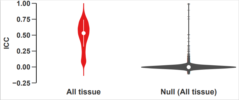

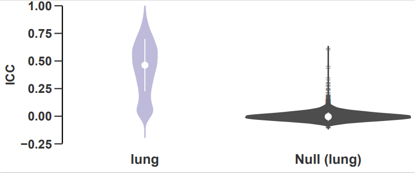
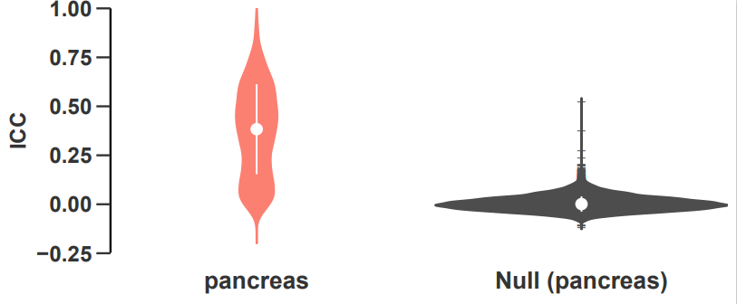
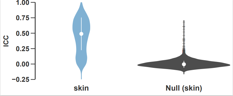
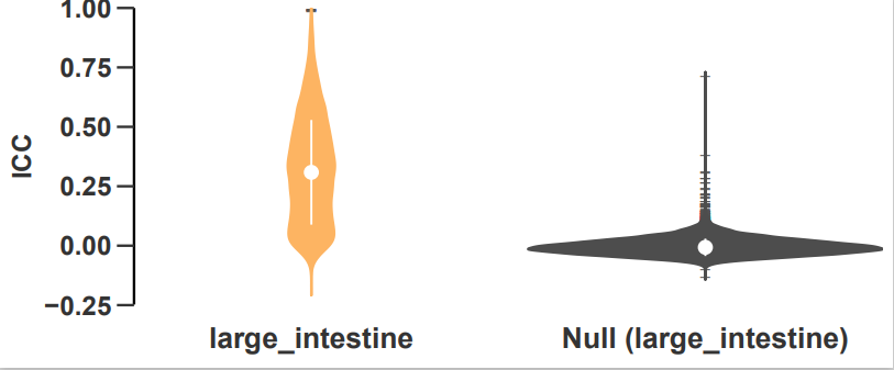
如图,小提琴图显示了所有样本的基因在PDX传代中的类内相关性(ICC),并按组织类型分层。黑色的小提琴图表示使用非传代相关(随机选择)样本计算的基因的ICC值。
小果以第一幅图为例子进行说明,这幅图显示了不同类型的肿瘤在通道之间的相关性。每种颜色代表一种特定类型的肿瘤。相关对的相关性的平均值是0.94,随机对的相关性的平均值是0.86,两者之间有显著的差异,这些图片可以帮助我们了解肿瘤的可塑性和适应性。
以上就是小果今天分享的全部内容啦,在今天的介绍中,我们通过使用Xeva包,对PDXE乳腺癌以及中基于PDX的药物进行了响应靶向通路的筛选,并且使用t-SNE对乳腺癌相关的数据进行了降维处理,最后通过分析说明PDX模型能够保持原始肿瘤的基因表达的稳定性和一致性,进而为精准医学的探索提供了良好的保障。
除了今天小果介绍的功能之外,Xeva包中还有很多的功能等着小伙伴们去探索,如果有其他生信方向的任何疑问,欢迎大家关注小果,试一试我们的云生信小工具,只要输入合适的数据,就可以直接绘制想要的图呢,链接:http://www.biocloudservice.com/home.html。