CIBERSORT包:洞悉细胞免疫浸润的神奇工具!
免疫细胞是我们身体的护卫军,它们在体内巡游,寻找并清除病原体,保护我们免受感染。当我们感染或出现其他异常情况时,免疫细胞会被引导到相应的组织中,形成免疫浸润。免疫浸润是免疫系统响应的重要表现,对于疾病的发展和治疗具有重要影响。在肿瘤中,免疫细胞的浸润情况尤其重要。一方面,免疫细胞的浸润可以帮助清除肿瘤细胞,起到抗肿瘤作用。另一方面,某些肿瘤可能通过操纵免疫系统,逃避免疫细胞的攻击,从而促进肿瘤的生长和转移。因此,准确了解免疫细胞在肿瘤组织中的分布和作用,对于肿瘤治疗和预后评估非常重要。
CIBERSORT是一个强大的生物信息学工具,由斯坦福大学的研究团队开发。它利用RNA测序数据,通过解析免疫基因表达谱,估算不同免疫细胞在样本中的比例。使用CIBERSORT,我们可以精准地了解组织中不同类型免疫细胞的分布情况,洞悉免疫浸润的奥秘。CIBERSORTx来自官网(https://cibersortx.stanford.edu/)的分析流程如图所示:
CIBERSORTx分析流程

如何使用CIBERSORT?使用CIBERSORT非常简单!让我为大家展示一下:
代码具体包括:
Step1 分析患者和对照样本的浸润程度
这里的LM22.txt 是CIBERSORT官方下载的文件,CIBERSORT_exp.txt是本地准备的基因表达文件,sampleName.csv是本地准备的样本信息文件,小果给大家附在最后。########分析患者和对照样本的浸润程度#加载包library(dplyr)library(tibble)library(tidyr)library(ggplot2)library(ggpubr)library(ggsci)library(reshape2)setwd("D:/wanglab/life/ziyuan/20230718/")# devtools::install_github("Moonerss/CIBERSORT")library(CIBERSORT)# 设置分析依赖的基础表达文件# 每类免疫细胞的标志性基因及其表达# 基因名字为Gene symbolLM22.file <- read.delim2("./LM22.txt",header = T)LM22.file[,-1] = lapply(LM22.file[,-1], FUN = function(y){as.numeric(y)})row.names(LM22.file) <- LM22.file$Gene.symbolLM22.file <- LM22.file[,-1]LM22.file <- as.matrix(LM22.file)#加载自己的数据用于分析计算免疫细胞load("GSE105450_raw.Rdata")#加载自己的数据用于分析计算免疫细胞# df <- express[,-c(1,2,4)]# #colnames(df)[1] <- "Gene symbol"# rownames(df) <- df$ORF# df <- df[,-1]df <- as.data.frame(express)write.table(df,"CIBERSORT_exp.txt",sep = "t",col.names = T,quote = F)df <- df[row.names(LM22.file),]TCGA_TME.results <- CIBERSORT::cibersort(LM22.file ,df, perm = 1000, QN = F)#perm置换次数=1000,QN分位数归一化=TRUE# perm置换次数=1000#输出结果write.csv(TCGA_TME.results, "./CIBERSORT_Results_fromRcode.csv")results <- TCGA_TME.results
Step2 箱线图展示
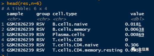
#########箱线图展示library(stringr)group <- sampleName$group[match(str_sub(colnames(df),1,10),sampleName$geo_accession)]group <- na.omit(group)res <- data.frame(results[,1:22])%>%dplyr::mutate(group = group)%>%tibble::rownames_to_column("sample")%>%tidyr::pivot_longer(cols = colnames(.)[2:23],names_to = "cell.type",values_to = 'value')head(res,n=6)
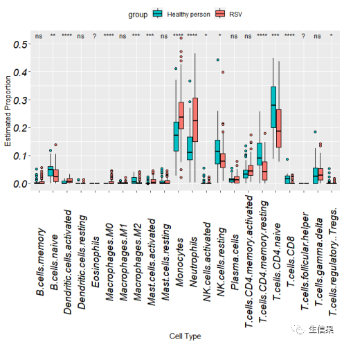
pdf(file = "CIBERSORT_psignif.pdf")ggplot(res,aes(cell.type,value,fill = group)) +geom_boxplot(outlier.shape = 21,color = "black",outlier.color = "black") +#theme_bw() +scale_fill_manual(values = c("#00BFC4","#F8766D"))+#设置颜色labs(x = "Cell Type", y = "Estimated Proportion") +theme(legend.position = "top") +theme(axis.text.x = element_text(angle=90,vjust = 0.5,size = 14,face = "italic",colour = 'black'),axis.text.y = element_text(face = "italic",size = 14,colour = 'black'))+#scale_fill_nejm()+stat_compare_means(aes(group = group),label = "p.signif",size=3,method = "kruskal.test")# p.format;p.signifdev.off()

免疫浸润结果箱线图比较
Step3 热图展示
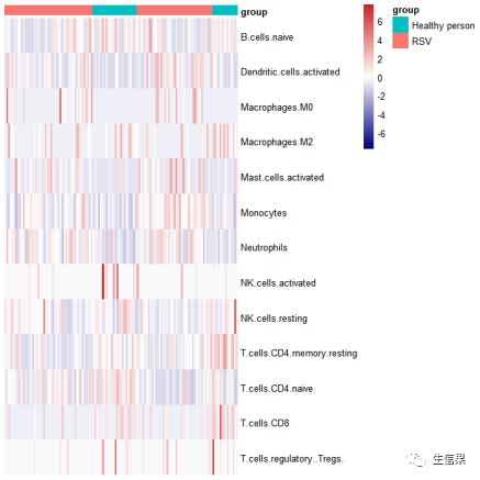
library(pheatmap)#选择具有差异性的免疫细胞deCell <- c("B.cells.naive","Dendritic.cells.activated","Macrophages.M0","Macrophages.M2","Mast.cells.activated","Monocytes","Neutrophils","NK.cells.activated","NK.cells.resting","T.cells.CD4.memory.resting","T.cells.CD4.naive","T.cells.CD8","T.cells.regulatory..Tregs.")TME.results <- TCGA_TME.resultsre <- TME.results[,-(23:25)]#展示差异的免疫细胞类型re2 <- as.data.frame(t(re[,deCell]))Group = grouptable(Group)an = data.frame(group = group,row.names = colnames(re2))groupcolor=c("#00BFC4","#F8766D")names(groupcolor)<- c("Healthy person","RSV")pdf(file="差异免疫细胞丰度热图.pdf")pheatmap::pheatmap(re2,scale = "row",show_colnames = F,cluster_rows = F,cluster_cols = F,annotation_col = an,annotation_colors = list(group=groupcolor),color = colorRampPalette(c("navy", "white", "firebrick3"))(50))dev.off()
差异免疫细胞丰度热图
希望通过这篇文章,你能对CIBERSORT有更深入的了解,并在生物信息学的世界里探索更多新奇的可能性。如果你对细胞组成的研究充满热情,那就赶快动手尝试一下CIBERSORT吧!
好了小果今天的分享就到这里了,小伙伴们,今天有没有学到新知识呢,想要继续了解R语言内容可以持续关注小果哦~或者也可以关注我们的官网也会持续更新的哦~
往期推荐