tidybulk—摈弃繁琐代码,在巨人肩膀学习转录组(一)
 相信各位进行生信研究的小伙伴们或多或少都听说过tidyverse这个R包,tidy主打一个简单快捷,小果之前还介绍过tidymodel包,是一个关于机器学习的R包,有兴趣的小伙伴可以在公众号进行搜索学习哦。言归正传,tidy是一个很重要的编程思想,在写代码的过程中,要求的就是减少代码的冗余和易读性。对于新入门的小伙伴而言更是如此,不仅可以帮助我们跑出结果增强自信心,还可以减轻我们学习大量代码所花费的时间。而今天小果给大家分享的也是tidy系列的一款R包,而这个R包主要的方向便是转录组的分析流程,而这个包就是tidybulk!小果也明白现在大家的研究热点都在单细胞的转录组分析,但在学习单细胞转录组之前,学习了解bulk转录组是能很好的奠定基础的!因为两个组学的基调都是转录组分析,只不过单细胞转录组更为特殊一些,使用的具体算法不太一样,需要进行更换。那么背景知识小果就讲到这啦!接下让小果带领大家开始今天的学习吧!代码基本都来自tidybulk的官网(https://github.com/stemangiola/tidybulk),有兴趣的小伙伴也可以上官网看看哦。
安装与加载R包
if(!require(tidybulk)) BiocManager::install("tidybulk")library(tidyverse)library(tidybulk)library(SummarizedExperiment)
示例数据
首先先让我们一起来看看示例数据,在tidybulk包中,我们研究的对象都是SummarizedExperiment对象。
data(counts_SE)counts_SE# class: SummarizedExperiment# dim: 8513 48# metadata(0):# assays(1): count# rownames(8513): A1BG A1BG-AS1 ... ZZEF1 ZZZ3# rowData names(0):# colnames(48): SRR1740034 SRR1740035 ... SRR1740088 SRR1740089# colData names(5): Cell.type time condition batch factor_of_interestclass(counts_SE)# [1] "SummarizedExperiment"# attr(,"package")# [1] "SummarizedExperiment"
获取转录组分析流程的文献
通过get_bibliography()函数,可以直接输出分析流程中的文献,这对各位小伙伴撰写论文,或是进行深一层学习都是极其方便的一个功能。
counts_SE %>%get_bibliography()# @Article{tidybulk,# title = {tidybulk: an R tidy framework for modular transcriptomic data analysis},# author = {Stefano Mangiola and Ramyar Molania and Ruining Dong and Maria A. Doyle & Anthony T. Papenfuss},# journal = {Genome Biology},# year = {2021},# volume = {22},# number = {42},# url = {https://genomebiology.biomedcentral.com/articles/10.1186/s13059-020-02233-7},# }# @article{wickham2019welcome,# title={Welcome to the Tidyverse},# author={Wickham, Hadley and Averick, Mara and Bryan, Jennifer and Chang, Winston and McGowan, Lucy D'Agostino and Francois, Romain and Grolemund, Garrett and Hayes, Alex and Henry, Lionel and Hester, Jim and others},# journal={Journal of Open Source Software},# volume={4},# number={43},# pages={1686},# year={2019}# }
整合重复的转录本
在我们的研究中,我们时常会遇到基因名,ENSEMBLE编号等进行互换的情况,但大多数时候他们的关系并不是一一对应的。这种时候,我们就必须处理重复项,小果今天介绍的R包就有这么一个函数,aggregate_duplicates函数可以将tibble和列名作为参数进行整合,一起来看看下面的例子。
gene_name =rownames(counts_SE)counts_SE.aggr = counts_SE %>%aggregate_duplicates(.transcript = gene_name)dim(counts_SE)# [1] 8513 48dim(counts_SE.aggr)# [1] 8513 48通过维度的比较我们看不出差别,这是因为在这个示例中,小果使用的是行名,行名本来就是没有重复的咧,所以我们换个方法。这里小果取一个极端一点的例子哦,我们假设a,b,c,d是不同的编号,使用同样的方案进行整合gene_name =c("a","b","c",rep("d",8510))tmp = counts_SE %>%aggregate_duplicates(.transcript = gene_name)dim(tmp)# [1] 4 48
标准化
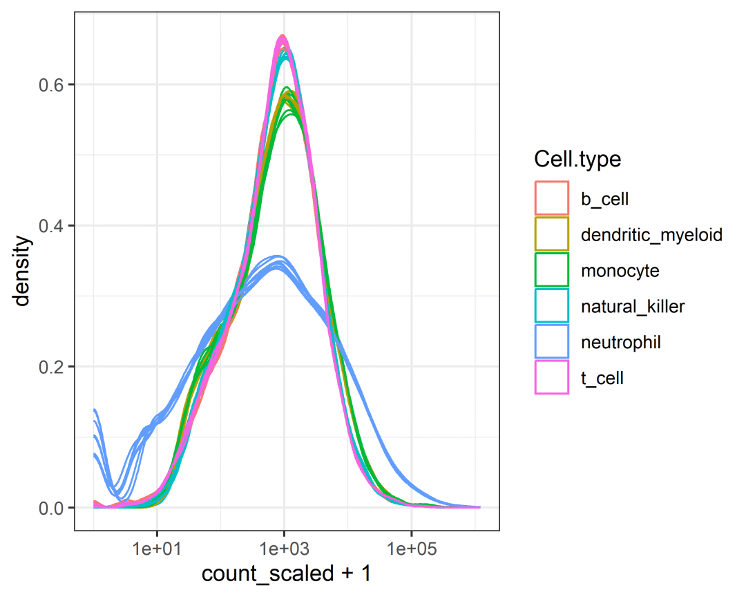
在转录组的分析过程中,我们需要将转录本的丰度进行标准化处理,这也是为了便于后续的分析处理。
小果这里解释一下代码哦~ 首先筛选出在不同条件下丰度显著不同的转录本,然后使用了scale_abundance()函数进行标准化。counts_SE.norm = counts_SE.aggr %>%identify_abundant(factor_of_interest = condition) %>%scale_abundance()assays(counts_SE.norm) %>%names()# [1] "count" "count_scaled"这里可以观察到,标准化过后增加了一个assay的矩阵assay(counts_SE.norm,"count_scaled")[1:5,1:5]# SRR1740034 SRR1740035 SRR1740036 SRR1740037 SRR1740038# A1BG 238.8192 312.8522 259.1186 206.4091 149.54205# A1BG-AS1 129.5555 134.4972 118.2644 124.1811 36.59008# AAAS 1354.8695 1478.0076 1360.7047 1246.8449 1094.52054# AACS 346.5219 400.5678 406.6168 354.0838 174.99602# AAGAB 920.9366 881.5416 968.7048 1023.6547 1374.51416小果通过这行代码将标准化过后的矩阵展现给各位小伙伴看看。tbl <- tidySummarizedExperiment::as_tibble(counts_SE.norm)这里小果自己遇到了一个bug哦,刚开始的时候一直转换不成功,经过研究后发现需要下载这个R包可以使用BiocManger进行下载哦BiocManager::install("tidySummarizedExperiment")head(tbl)# # A tibble: 6 × 13# .feature .sample count count_scaled Cell.type time condition batch## 1 A1BG SRR1740034 153 239. b_cell 0 d TRUE 0# 2 A1BG-AS1 SRR1740034 83 130. b_cell 0 d TRUE 0# 3 AAAS SRR1740034 868 1355. b_cell 0 d TRUE 0# 4 AACS SRR1740034 222 347. b_cell 0 d TRUE 0# 5 AAGAB SRR1740034 590 921. b_cell 0 d TRUE 0# 6 AAMDC SRR1740034 48 74.9 b_cell 0 d TRUE 0# # ℹ 5 more variables: factor_of_interest, TMM, multiplier,# # gene_name, .abundantnames(tbl)# [1] ".feature" ".sample" "count"# [4] "count_scaled" "Cell.type" "time"# [7] "condition" "batch" "factor_of_interest"# [10] "TMM" "multiplier" "gene_name"# [13] ".abundant"对标准化的结果进行可视化counts_SE.norm %>%ggplot(aes(count_scaled +1, group=.sample, color=Cell.type)) +geom_density() +scale_x_log10() +scale_fill_brewer(palette ="Set3") +theme_bw()
筛选变异基因
转录组的分析,我们首要的目的就是想找出差异嘛,而这一步就是筛选出差异基因。
counts_SE.norm.variable = counts_SE.norm %>%keep_variable(top =100) # 小果这里通过top参数仅保留了前100基因。head(counts_SE.norm.variable)# # A SummarizedExperiment-tibble abstraction: 288 × 48# # [90mFeatures=6 | Samples=48 | Assays=count, count_scaled[0m# .feature .sample count count_scaled Cell.type time condition batch## 1 SERPINA1 SRR1740034 4 6.24 b_cell 0 d TRUE 0# 2 CSF3R SRR1740034 4 6.24 b_cell 0 d TRUE 0# 3 TNFAIP2 SRR1740034 4 6.24 b_cell 0 d TRUE 0# 4 S100A9 SRR1740034 16 25.0 b_cell 0 d TRUE 0# 5 VCAN SRR1740034 8 12.5 b_cell 0 d TRUE 0# 6 C5AR1 SRR1740034 2 3.12 b_cell 0 d TRUE 0# 7 SERPINA1 SRR1740035 4 5.85 b_cell 1 d TRUE 1# 8 CSF3R SRR1740035 12 17.5 b_cell 1 d TRUE 1# 9 TNFAIP2 SRR1740035 11 16.1 b_cell 1 d TRUE 1# 10 S100A9 SRR1740035 15 21.9 b_cell 1 d TRUE 1# # ℹ 110 more rows# # ℹ 5 more variables: factor_of_interest, TMM, multiplier,# # gene_name, .abundant

降维
tidybulk包中集合了三种降维的算法,他们分别是MDS,PCA和tSNE,各位小伙伴可以根据需求进行选择。小果在这对三种算法都进行一遍演示。## MDS
counts_SE.norm.MDS =counts_SE.norm %>%reduce_dimensions(method="MDS", .dims =6)counts_SE.norm.MDS %>%pivot_sample() %>%# 保留样本相关的列,这样可以减少计算的时间。select(contains("Dim"), everything()) # 通过这行代码可以减少列的顺序。# # A tibble: 48 × 14# Dim1 Dim2 Dim3 Dim4 Dim5 Dim6 .sample Cell.type time## 1 -1.46 0.220 -1.68 0.0553 0.0658 -0.126 SRR1740034 b_cell 0 d# 2 -1.46 0.226 -1.71 0.0300 0.0454 -0.137 SRR1740035 b_cell 1 d# 3 -1.44 0.193 -1.60 0.0890 0.0503 -0.121 SRR1740036 b_cell 3 d# 4 -1.44 0.198 -1.67 0.0891 0.0543 -0.110 SRR1740037 b_cell 7 d# 5 0.243 -1.42 0.182 0.00642 -0.503 -0.131 SRR1740038 dendritic_mye… 0 d# 6 0.191 -1.42 0.195 0.0180 -0.457 -0.130 SRR1740039 dendritic_mye… 1 d# 7 0.257 -1.42 0.152 0.0130 -0.582 -0.0927 SRR1740040 dendritic_mye… 3 d# 8 0.162 -1.43 0.189 0.0232 -0.452 -0.109 SRR1740041 dendritic_mye… 7 d# 9 0.516 -1.47 0.240 -0.251 0.457 -0.119 SRR1740042 monocyte 0 d# 10 0.514 -1.41 0.231 -0.219 0.458 -0.131 SRR1740043 monocyte 1 d# # ℹ 38 more rows# # ℹ 5 more variables: condition, batch, factor_of_interest,# # TMM, multiplier小果小Tips:在这需要安装一个R包哦~# install.packages("GGally")counts_SE.norm.MDS %>%pivot_sample() %>%GGally::ggpairs(columns =6:(6+5), ggplot2::aes(colour=`Cell.type`))
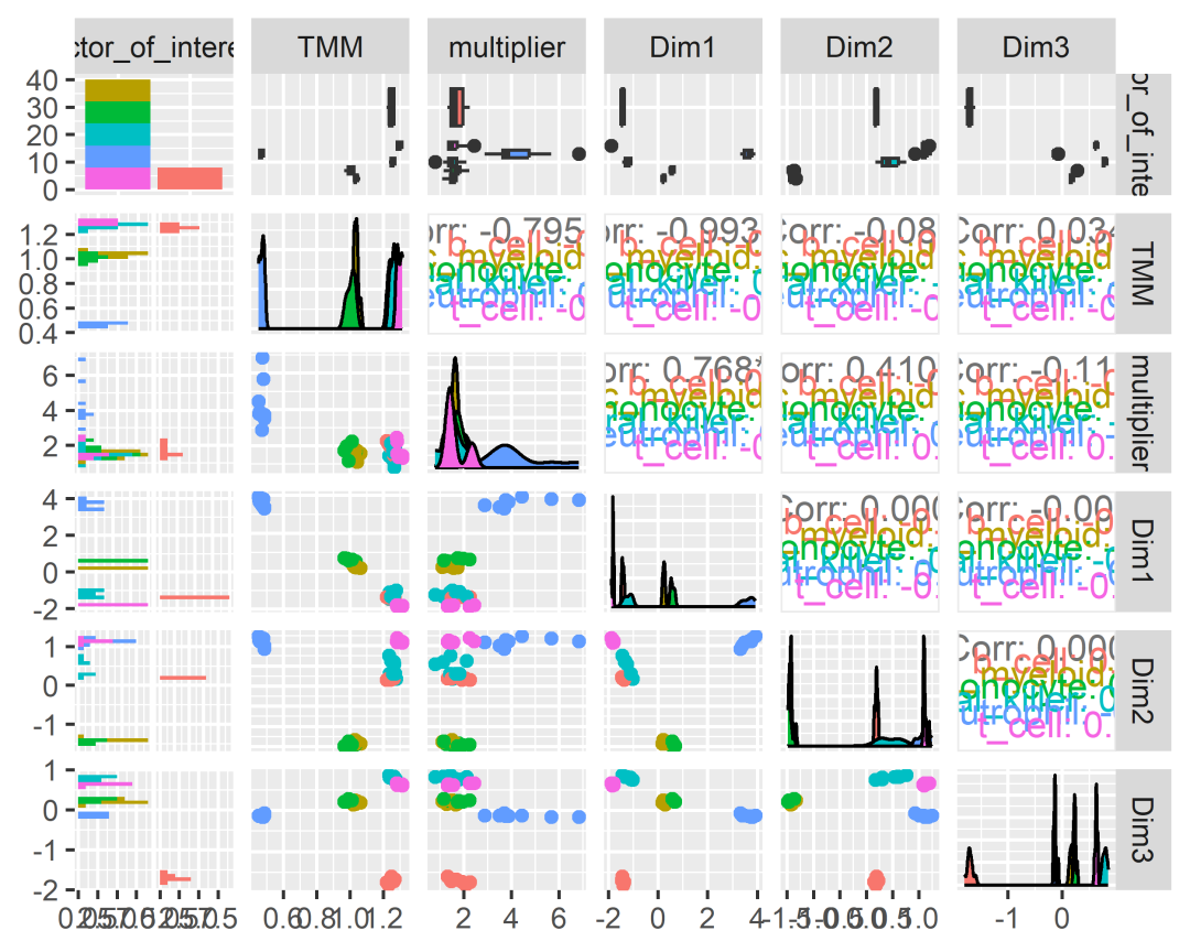
# 这个图就是各维度之间的相关关系啦PCA
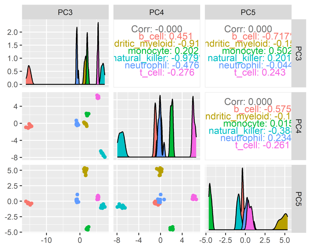
counts_SE.norm.PCA =counts_SE.norm %>%reduce_dimensions(method="PCA", .dims =6)counts_SE.norm.PCA %>%pivot_sample() %>%select(contains("PC"), everything())# # A tibble: 48 × 14# PC1 PC2 PC3 PC4 PC5 PC6 .sample Cell.type time condition## 1 -12.6 -2.52 -14.9 -0.424 -0.592 -1.22 SRR17400… b_cell 0 d TRUE# 2 -12.6 -2.57 -15.2 -0.140 -0.388 -1.30 SRR17400… b_cell 1 d TRUE# 3 -12.6 -2.41 -14.5 -0.714 -0.344 -1.10 SRR17400… b_cell 3 d TRUE# 4 -12.5 -2.34 -14.9 -0.816 -0.427 -1.00 SRR17400… b_cell 7 d TRUE# 5 0.189 13.0 1.66 -0.0269 4.64 -1.35 SRR17400… dendriti… 0 d FALSE# 6 -0.293 12.9 1.76 -0.0727 4.21 -1.28 SRR17400… dendriti… 1 d FALSE# 7 0.407 13.0 1.42 -0.0529 5.37 -1.01 SRR17400… dendriti… 3 d FALSE# 8 -0.620 13.0 1.73 -0.201 4.17 -1.07 SRR17400… dendriti… 7 d FALSE# 9 2.56 13.5 2.32 2.03 -4.32 -1.22 SRR17400… monocyte 0 d FALSE# 10 2.65 13.1 2.21 1.80 -4.29 -1.30 SRR17400… monocyte 1 d FALSE# # ℹ 38 more rows# # ℹ 4 more variables: batch, factor_of_interest, TMM,# # multipliercounts_SE.norm.PCA %>%pivot_sample() %>%GGally::ggpairs(columns =11:13, ggplot2::aes(colour=`Cell.type`))
tSNE
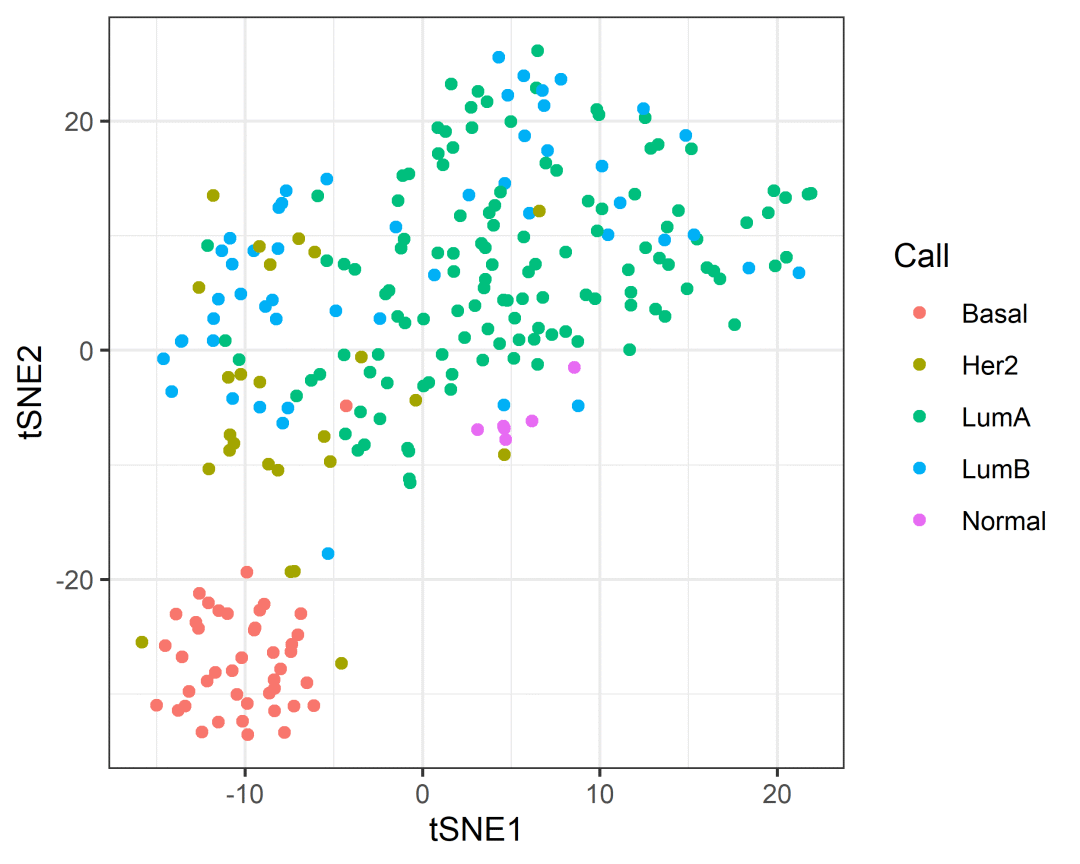
counts_SE.norm.tSNE =breast_tcga_mini_SE %>%identify_abundant() %>%# 筛选高表达的特异基因reduce_dimensions(method ="tSNE",perplexity=10,pca_scale =TRUE)# Performing PCA# Read the 251 x 50 data matrix successfully!# OpenMP is working. 1 threads.# Using no_dims = 2, perplexity = 10.000000, and theta = 0.500000# Computing input similarities...# Building tree...# Done in 0.02 seconds (sparsity = 0.182886)!# Learning embedding...# Iteration 50: error is 67.381499 (50 iterations in 0.03 seconds)# Iteration 100: error is 68.239243 (50 iterations in 0.04 seconds)# Iteration 150: error is 69.030962 (50 iterations in 0.03 seconds)# Iteration 200: error is 69.041501 (50 iterations in 0.04 seconds)# Iteration 250: error is 67.702680 (50 iterations in 0.05 seconds)# Iteration 300: error is 1.540607 (50 iterations in 0.04 seconds)# Iteration 350: error is 1.193476 (50 iterations in 0.02 seconds)# Iteration 400: error is 1.146808 (50 iterations in 0.02 seconds)# Iteration 450: error is 1.135869 (50 iterations in 0.02 seconds)# Iteration 500: error is 1.121872 (50 iterations in 0.01 seconds)# Iteration 550: error is 1.119940 (50 iterations in 0.01 seconds)# Iteration 600: error is 1.115307 (50 iterations in 0.01 seconds)# Iteration 650: error is 1.110707 (50 iterations in 0.01 seconds)# Iteration 700: error is 1.108459 (50 iterations in 0.01 seconds)# Iteration 750: error is 1.102872 (50 iterations in 0.01 seconds)# Iteration 800: error is 1.099258 (50 iterations in 0.02 seconds)# Iteration 850: error is 1.095792 (50 iterations in 0.01 seconds)# Iteration 900: error is 1.093945 (50 iterations in 0.01 seconds)# Iteration 950: error is 1.092175 (50 iterations in 0.01 seconds)# Iteration 1000: error is 1.091423 (50 iterations in 0.01 seconds)# Fitting performed in 0.44 seconds.counts_SE.norm.tSNE %>%pivot_sample() %>%select(contains("tSNE"), everything())# # A tibble: 251 × 4# tSNE1 tSNE2 .sample Call## 1 3.33 9.32 TCGA-A1-A0SD-01A-11R-A115-07 LumA# 2 -3.49 -5.36 TCGA-A1-A0SF-01A-11R-A144-07 LumA# 3 -0.759 15.4 TCGA-A1-A0SG-01A-11R-A144-07 LumA# 4 -3.82 7.05 TCGA-A1-A0SH-01A-11R-A084-07 LumA# 5 0.670 6.59 TCGA-A1-A0SI-01A-11R-A144-07 LumB# 6 -1.38 13.0 TCGA-A1-A0SJ-01A-11R-A084-07 LumA# 7 -9.85 -33.5 TCGA-A1-A0SK-01A-12R-A084-07 Basal# 8 -12.1 9.13 TCGA-A1-A0SM-01A-11R-A084-07 LumA# 9 -10.9 9.79 TCGA-A1-A0SN-01A-11R-A144-07 LumB# 10 1.61 23.2 TCGA-A1-A0SQ-01A-21R-A144-07 LumA# # ℹ 241 more rowscounts_SE.norm.tSNE %>%pivot_sample() %>%ggplot(aes(x =`tSNE1`, y =`tSNE2`, color=Call)) +geom_point() +theme_bw()
 这以上就是转录组分析的前半部分的分析流程啦,内容也有点多,小果会分为两章进行讲诉哦~也希望各位小伙伴可以咀嚼吸收,关注我们的公众号发文,给大家稍微剧透一下,在后半章小果会教大家丰度差异,机器学习推断细胞组成等等内容,敬请期待哦!


往期推荐