2024-06-16

想在一张图中进多种数据展示方法？看看gghalves包

小图生信果 2023-09-04 19:02:21

转自公众号：生信图
http://mp.weixin.qq.com/s?__biz=MzkxODUxNDgzNA==&mid=2247484801&idx=1&sn=b0829415b781e32177a1331496a9d5f1

点击蓝字

关注小图

在我们的研究中，我们经常需要对数据的分布进行展示，而其中我们最常用的数据分布可视化和统计信息的图表有三种，那就是Boxplot，volinplot和Pointplot。但这三个图具有不同的优点，小伙伴有没有试想过，画一个具有所有图表优势的图呢？今天小图介绍的R包就可以让我们在一张图表中具有所有优势，那就是gghalves包。 gghalves包可以通过ggplot2轻松编写自己的一半一半情节。想想在抖动点旁边显示一个箱形图，或者在点图旁边显示小提琴图。通过同时展示三种类型的图，通过箱线图显示数据的五数概括（最小值、第一四分位数、中位数、第三四分位数和最大值）来展示数据分布，看出中心趋势和离散度；通过小提琴图展示更详细的分布情况；通过点图，可以展示各个数据点的分布情况，以及平均值、置信区间等统计信息。

step0 安装与加载

options(timeout = 999)
if (!require(devtools)) {  install.packages('devtools')}## 载入需要的程辑包：devtools## 载入需要的程辑包：usethisif (!require(gghalves)) {  devtools::install_github('erocoar/gghalves')}## 载入需要的程辑包：gghalves## 载入需要的程辑包：ggplot2## Warning: 程辑包'ggplot2'是用R版本4.2.3 来建造的library(gghalves)

step1 模拟数据

# 设置随机数种子以确保结果可重复set.seed(123)
# 生成随机数据num_samples <- 50
custom_iris <- data.frame(  S.Length = runif(num_samples, 4.0, 8),  S.Width = runif(num_samples, 2.0, 5),  P.Length = runif(num_samples, 1.0, 6.0),  P.Width = runif(num_samples, 0.1, 3),  Species = sample(c("S1", "S2", "S3"), num_samples, replace = TRUE))

step2 功能预览

gghalves包中包含了三个主要的函数 geom_half_point、geom_half_boxplot、 geom_half_violin

geom_half_point

我们先来看看对比

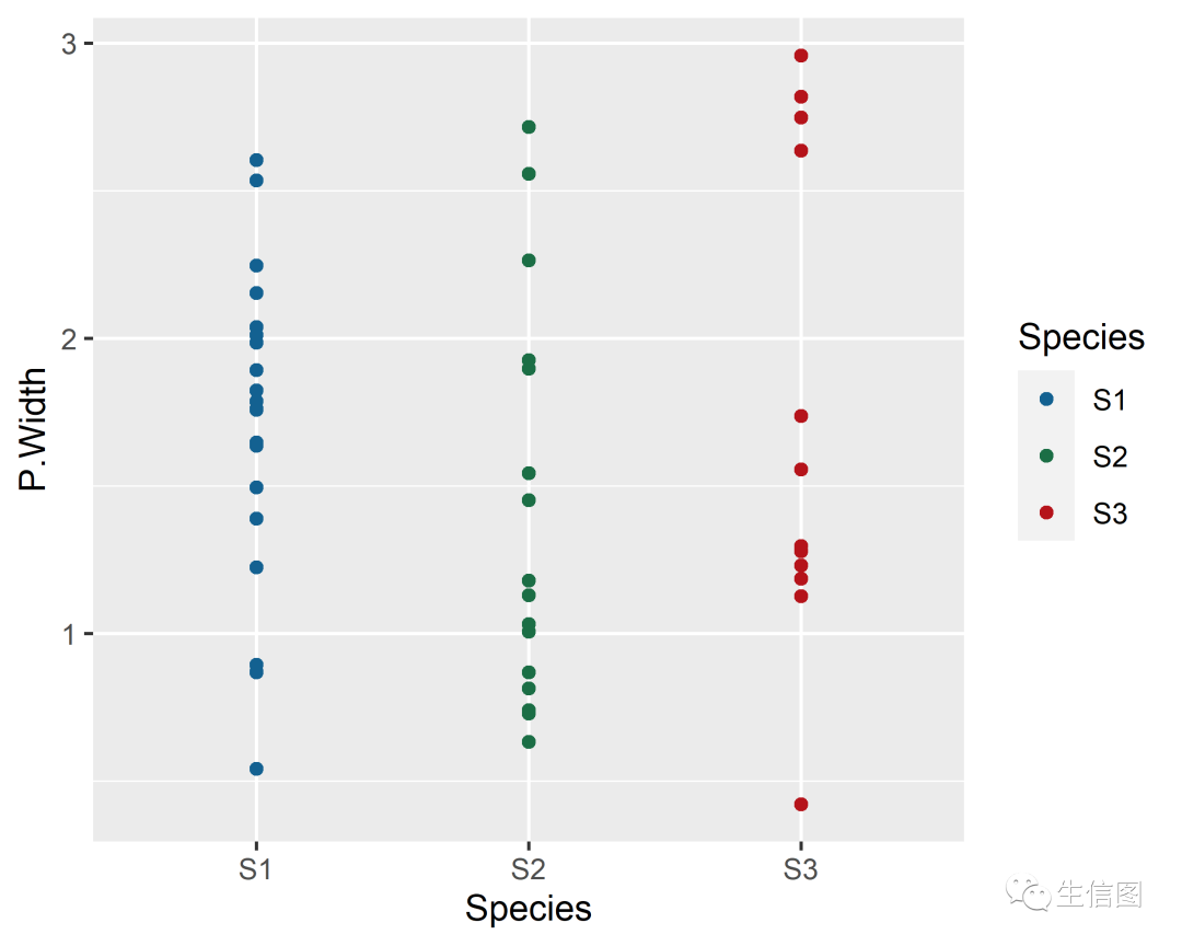
ggplot(custom_iris, aes(x = Species, y = P.Width, color = Species)) +   scale_color_manual(values = c("#136191", "#1b6e45","#b5131a"))+    geom_point()

ggplot(custom_iris, aes(x = Species, y = P.Width, color = Species)) +   scale_color_manual(values = c("#136191", "#1b6e45","#b5131a"))+    geom_half_point()

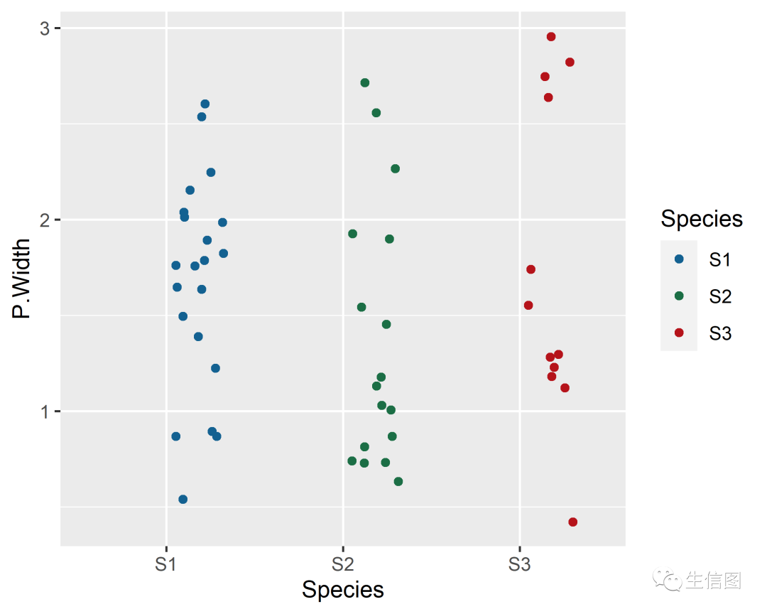
出点图只占了一半，左半部分或右半部分留给另一个geom使用，geom_half_point函数会添加水平和垂直抖动点。

geom_half_boxplot

ggplot(custom_iris, aes(x = Species, y = P.Width, fill = Species)) +   scale_fill_manual(values = c("#136191", "#1b6e45","#b5131a"))+    geom_half_boxplot()

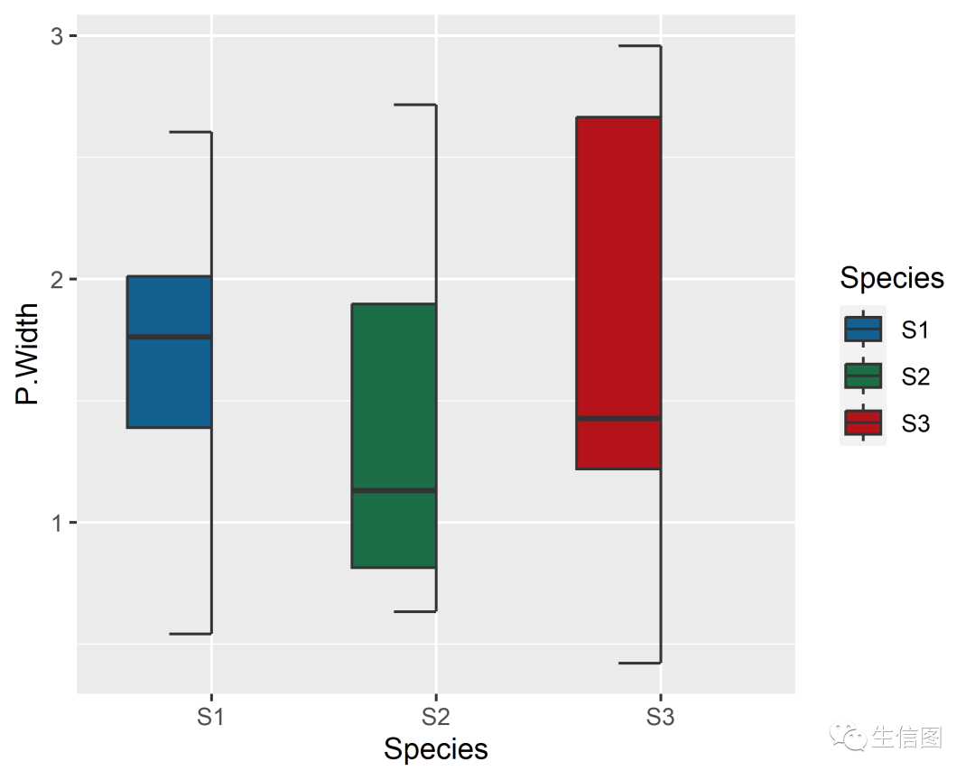
ggplot(custom_iris, aes(x = Species, y = P.Width, fill = Species)) +   scale_fill_manual(values = c("#136191", "#1b6e45","#b5131a"))+    geom_half_boxplot(center = T) # 使用center参数可以将箱线图居中展示

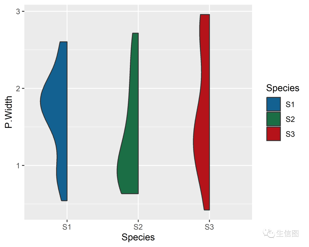
geom_half_violin

ggplot(custom_iris, aes(x = Species, y = P.Width, fill = Species)) +   scale_fill_manual(values = c("#136191", "#1b6e45","#b5131a"))+    geom_half_violin()

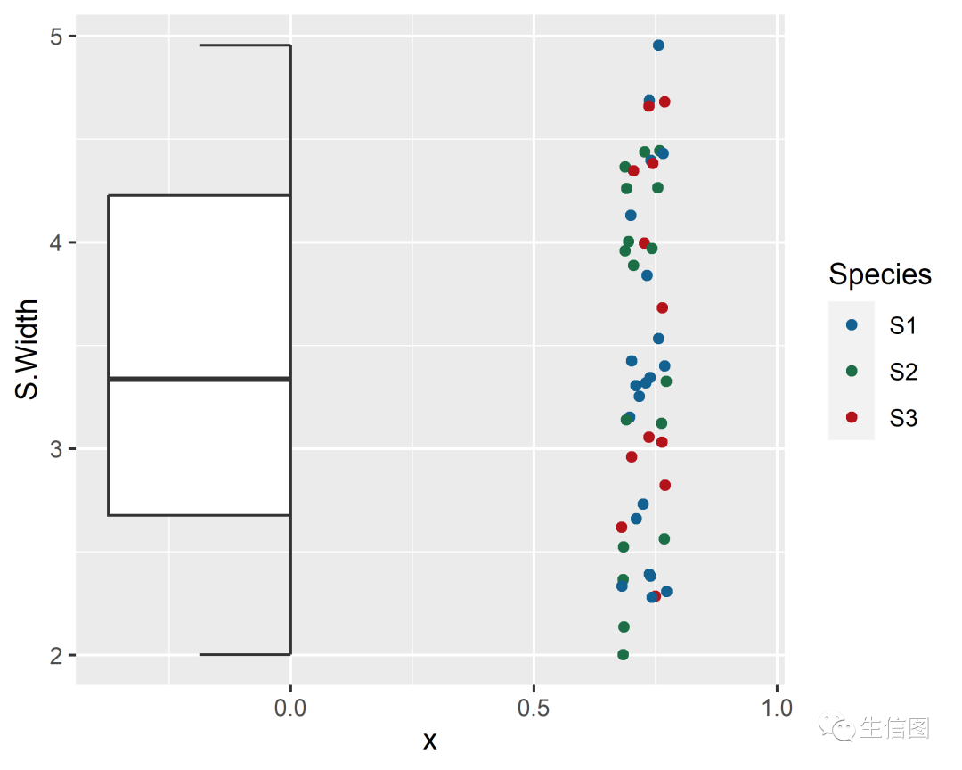
geom_half_point_panel

geom_half_point_panel函数可以将不同类型的数据展示图分半进行展示。ggplot(custom_iris, aes(y = S.Width)) +  geom_half_boxplot() +  geom_half_point_panel(aes(x = 0.5, color = Species), range_scale = .5) +  scale_color_manual(values = c("#136191", "#1b6e45","#b5131a"))

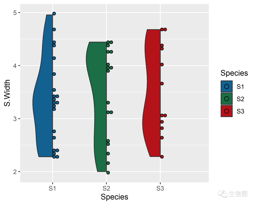
GeomHalfDotplot

除了以上的基础图形以外，还有一个内置的半点图。ggplot(custom_iris, aes(x = Species, y = S.Width, fill = Species)) +  geom_half_violin() +   geom_dotplot(binaxis = "y", method="histodot", stackdir="up",binwidth=0.06) +  scale_fill_manual(values = c("#136191", "#1b6e45","#b5131a"))

组合图形

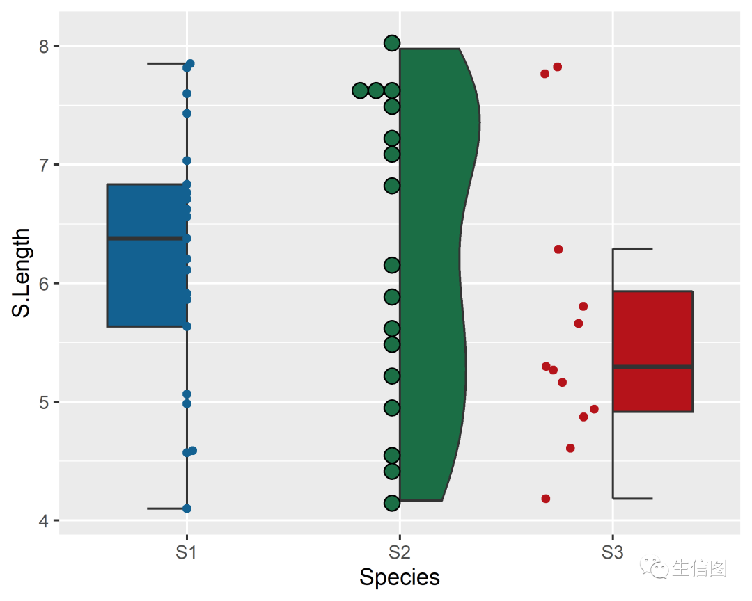
跟着小图了解了那么多不同类型的可视化图后，不知道大家是否清楚怎么使用了呢？来和小图一起将上面学的图面都使用起来，绘制在同一张图上。

小图小Tips：通过side参数，我们可以调整半图所在的位置 “r”–右边，“l”–左边。

library(tidyverse)## Warning: 程辑包'tidyverse'是用R版本4.2.3 来建造的## Warning: 程辑包'tibble'是用R版本4.2.3 来建造的## Warning: 程辑包'dplyr'是用R版本4.2.3 来建造的## ── Attaching core tidyverse packages ──────────────────────── tidyverse 2.0.0 ──## ✔ dplyr     1.1.2     ✔ readr     2.1.4## ✔ forcats   1.0.0     ✔ stringr   1.5.0## ✔ lubridate 1.9.2     ✔ tibble    3.2.1## ✔ purrr     1.0.1     ✔ tidyr     1.3.0## ── Conflicts ────────────────────────────────────────── tidyverse_conflicts() ──## ✖ dplyr::filter() masks stats::filter()## ✖ dplyr::lag()    masks stats::lag()## ℹ Use the conflicted package (<http://conflicted.r-lib.org/>) to force all conflicts to become errorsggplot() +  # S1组箱图+点图  geom_half_boxplot(    data = custom_iris %>% filter(Species=="S1"),     aes(x = Species, y = S.Length, fill = Species), outlier.color = NA) +  ggbeeswarm::geom_beeswarm(    data = custom_iris %>% filter(Species=="S1"),    aes(x = Species, y = S.Length, fill = Species, color = Species), beeswarmArgs=list(side=+1)) +  # S2组 使用了GeomHalfDotplot  geom_half_violin(    data = custom_iris %>% filter(Species=="S2"),     aes(x = Species, y = S.Length, fill = Species), side="r") +    geom_half_dotplot(    data = custom_iris %>% filter(Species=="S2"),     aes(x = Species, y = S.Length, fill = Species), method="histodot", stackdir="down") +  #   geom_half_boxplot(    data = custom_iris %>% filter(Species=="S3"),     aes(x = Species, y = S.Length, fill = Species), side = "r", errorbar.draw = TRUE,    outlier.color = NA) +    geom_half_point(    data = custom_iris %>% filter(Species=="S3"),     aes(x = Species, y = S.Length, fill = Species, color = Species), side = "l") +    scale_fill_manual(values = c("S1" = "#136191", "S2"="#1b6e45","S3"="#b5131a")) +  scale_color_manual(values = c("S1" = "#136191", "S2"="#1b6e45","S3"="#b5131a")) +  theme(legend.position = "none")## Warning: The `beeswarmArgs` argument of `geom_beeswarm()` is deprecated as of ggbeeswarm## 0.7.1.## This warning is displayed once every 8 hours.## Call `lifecycle::last_lifecycle_warnings()` to see where this warning was## generated.## Bin width defaults to 1/30 of the range of the data. Pick better value with## `binwidth`.

step3 进阶图形

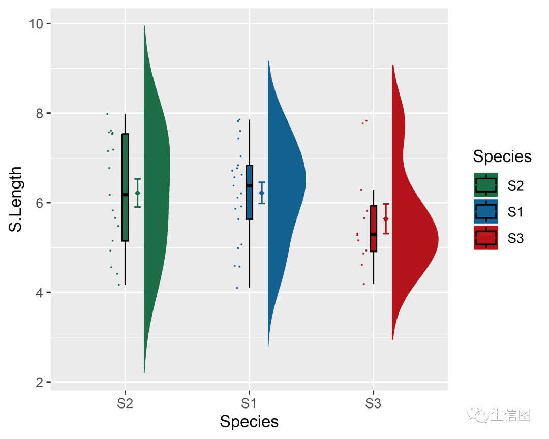
云雨图

我们先对数据进行统计学计算，包含了均值，标准差，数量标准误差。

# 统计摘要summ_iris <- custom_iris %>%     group_by(Species) %>%     summarise(        mean = mean(S.Length),        sd = sd(S.Length),        n = n()    ) %>%     mutate(se = sd/sqrt(n),                 Species = factor(Species, levels = c('S2', 'S1', 'S3')))summ_iris## # A tibble: 3 × 5##   Species  mean    sd     n    se##   <fct>   <dbl> <dbl> <int> <dbl>## 1 S1       6.22  1.09    21 0.238## 2 S2       6.22  1.29    17 0.312## 3 S3       5.64  1.15    12 0.331# 数据转换  iris_plot <- custom_iris %>%     mutate(Species = factor(Species, levels = c('S2', 'S1', 'S3')))head(iris_plot)##   S.Length  S.Width P.Length   P.Width Species## 1 5.150310 2.137494 3.999945 2.5576142      S2## 2 7.153221 3.326600 2.664118 1.5428291      S2## 3 5.635908 4.396775 3.443065 1.2249362      S1## 4 7.532070 2.365698 5.772369 0.8147021      S2## 5 7.761869 3.682844 3.414512 0.4221797      S3## 6 4.182226 2.619594 5.451751 1.2309839      S3# 使用ggpubr包的geom_signif加入显著性结果library(ggpubr)library(ggsci)## Warning: 程辑包'ggsci'是用R版本4.2.3 来建造的# 绘图ggplot(iris_plot , aes(x = Species, y = S.Length, fill = Species))+    geom_half_violin(aes(fill = Species),                                     position = position_nudge(x = .15, y = 0),                                     adjust=1.5, trim=FALSE, colour=NA, side = 'r') +    geom_point(aes(x = as.numeric(Species)-0.1,                                 y = S.Length,color = Species),                         position = position_jitter(width = .05),size = .25, shape = 20) +    geom_boxplot(aes(x = Species,y = S.Length, fill = Species),                             outlier.shape = NA,                             width = .05,                             color = "black")+    geom_point(data=summ_iris,                         aes(x=Species,y = mean, group = Species, color = Species),                         shape=18,                         size = 1.5,                         position = position_nudge(x = .1,y = 0)) +    geom_errorbar(data = summ_iris,                                aes(x = Species, y = mean, group = Species, colour = Species,                                        ymin = mean-se, ymax = mean+se),                                width=.05,                                position=position_nudge(x = .1, y = 0)    ) +    scale_color_manual(values = c("S1" = "#136191", "S2"="#1b6e45","S3"="#b5131a")) +    scale_fill_manual(values = c("S1" = "#136191", "S2"="#1b6e45","S3"="#b5131a"))