2024-06-16

探索基因共表达网络：WGCNA揭示基因调控网络的奥秘

小花生信果 2023-08-24 19:00:10

转自公众号：生信花
http://mp.weixin.qq.com/s?__biz=MzkzODUxNjcwMA==&mid=2247484252&idx=1&sn=a778d2dea96f118f0e31ee09f982a1a5

点击蓝字关注我们

引言：

随着高通量测序技术的快速发展，我们能够获取大量基因表达数据，这为我们深入理解基因调控网络提供了巨大的机会。然而，如何从这些海量数据中提取有意义的信息仍然是一个挑战。在这方面，WGCNA成为了研究人员的得力工具，帮助我们揭示基因共表达模式、发现关键调控基因以及了解基因调控网络的功能。

WGCNA原理：

WGCNA基于基因共表达模式，即具有相似表达模式的基因倾向于在生物学功能和调控网络中具有相似的角色。该方法通过构建基因共表达网络，将高度相关的基因聚合成共表达模块，并通过模块间和模块内的连接强度来鉴定关键基因。WGCNA还使用系统生物学和网络理论的原理来揭示基因调控网络的功能和机制。

应用领域：

WGCNA广泛应用于生物学研究的多个领域。在癌症研究中，研究人员利用WGCNA分析肿瘤组织和正常组织的基因表达数据，发现了与癌症相关的共表达模块和关键调控基因。在植物研究中，WGCNA帮助揭示了植物发育和抗逆性的基因调控网络。此外，WGCNA在神经科学、免疫学、代谢组学等领域也有广泛应用。

分析步骤：

使用WGCNA进行基因共表达网络分析通常包括以下步骤：

1）数据预处理，包括数据清洗、标准化和选择感兴趣的基因集

2）构建相关系数矩阵，计算基因间的相关性

3）构建基因共表达网络，通过选择合适的相似性度量和连接阈值

4）模块发现，将高度相关的基因聚合成共表达模块

5）模块的功能注释和调控基因的识别

6）网络可视化和功能分析

下面我们以肝癌数据为例进行分析：

注：这里的”LiverFemale3600.csv”,”ClinicalTraits.csv”是自行准备的本地文件，小花给大家附在最后。

Step1 数据输入、清洗和预处理

# 1.1 载入数据workingDir = "D:/wanglab/life/ziyuan/WGCNA/";setwd(workingDir);# Load the WGCNA packagelibrary(WGCNA);# The following setting is important, do not omit.options(stringsAsFactors = FALSE);#Read in the female liver data setfemData = read.csv("LiverFemale3600.csv");# Take a quick look at what is in the data set:dim(femData);names(femData);#1.2创建行为样本，列为基因的表达矩阵datExpr0 = as.data.frame(t(femData[, -c(1:8)]));names(datExpr0) = femData$substanceBXH;rownames(datExpr0) = names(femData)[-c(1:8)];### 1.3判断数据质量--缺失值gsg = goodSamplesGenes(datExpr0, verbose = 3);gsg$allOKif (!gsg$allOK){# Optionally, print the gene and sample names that were removed:if (sum(!gsg$goodGenes)>0)printFlush(paste("Removing genes:", paste(names(datExpr0)[!gsg$goodGenes], collapse = ", ")));if (sum(!gsg$goodSamples)>0)printFlush(paste("Removing samples:", paste(rownames(datExpr0)[!gsg$goodSamples], collapse = ", ")));# Remove the offending genes and samples from the data:datExpr0 = datExpr0[gsg$goodSamples, gsg$goodGenes]}### 1.4绘制样品的系统聚类树sampleTree = hclust(dist(datExpr0), method = "average");# Plot the sample tree: Open a graphic output window of size 12 by 9 inches# The user should change the dimensions if the window is too large or too small.sizeGrWindow(12,9)#pdf(file = "Plots/sampleClustering.pdf", width = 12, height = 9);par(cex = 0.6);par(mar = c(0,4,2,0))plot(sampleTree, main = "Sample clustering to detect outliers", sub="", xlab="", cex.lab = 1.5,cex.axis = 1.5, cex.main = 2)# Plot a line to show the cutabline(h = 15, col = "red");

绘制样本树聚类树

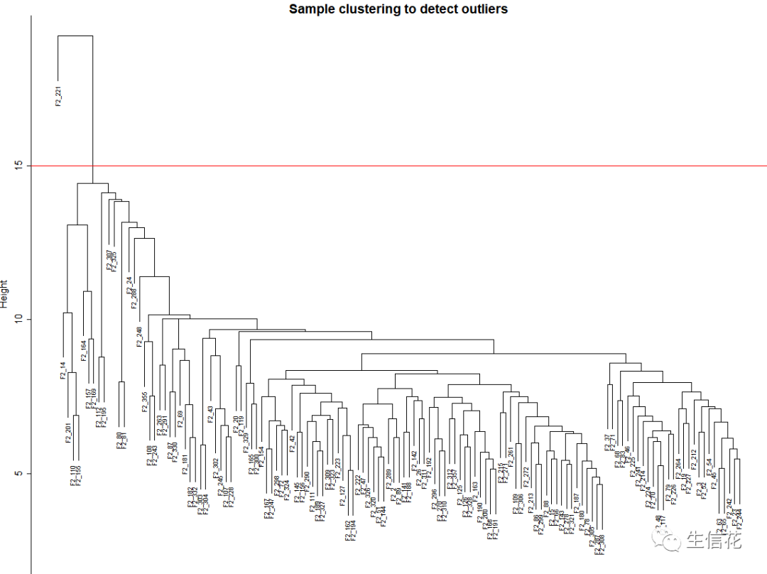
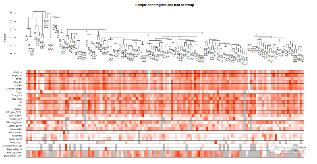
## 1.5若存在显著离群点；剔除掉# Determine cluster under the lineclust = cutreeStatic(sampleTree, cutHeight = 15, minSize = 10)table(clust)# clust 1 contains the samples we want to keep.keepSamples = (clust==1)datExpr = datExpr0[keepSamples, ]nGenes = ncol(datExpr)nSamples = nrow(datExpr)rownames(datExpr0)[!keepSamples]### 1.6读入临床表型数据traitData = read.csv("ClinicalTraits.csv");dim(traitData)names(traitData)# remove columns that hold information we do not need.allTraits = traitData[, -c(31, 16)];allTraits = allTraits[, c(2, 11:36) ];dim(allTraits)names(allTraits)# Form a data frame analogous to expression data that will hold the clinical traits.femaleSamples = rownames(datExpr);traitRows = match(femaleSamples, allTraits$Mice);datTraits = allTraits[traitRows, -1];rownames(datTraits) = allTraits[traitRows, 1];collectGarbage();### 1.7再次对删掉离群值的样本进行聚类# Re-cluster samplessampleTree2 = hclust(dist(datExpr), method = "average")# Convert traits to a color representation: white means low, red means high, grey means missing entrytraitColors = numbers2colors(datTraits, signed = FALSE);# Plot the sample dendrogram and the colors underneath.plotDendroAndColors(sampleTree2, traitColors,groupLabels = names(datTraits),main = "Sample dendrogram and trait heatmap")

绘制样本树聚类树和表型热图

### 1.8保存表型和基因表达数据，以便后续分析save(datExpr, datTraits, file = "FemaleLiver-01-dataInput.RData")

Step2网络搭建及模块检测

### 2.1 挑选最佳阈值power# Load the data saved in the first partlnames = load(file = "FemaleLiver-01-dataInput.RData");#The variable lnames contains the names of loaded variables.lnames# Choose a set of soft-thresholding powerspowers = c(c(1:10), seq(from = 12, to=20, by=2))# Call the network topology analysis functionsft = pickSoftThreshold(datExpr, powerVector = powers, verbose = 5)# Plot the results:sizeGrWindow(9, 5)par(mfrow = c(1,2));cex1 = 0.9;# Scale-free topology fit index as a function of the soft-thresholding powerplot(sft$fitIndices[,1], -sign(sft$fitIndices[,3])*sft$fitIndices[,2],xlab="Soft Threshold (power)",ylab="Scale Free Topology Model Fit,signed R^2",type="n",main = paste("Scale independence"));text(sft$fitIndices[,1], -sign(sft$fitIndices[,3])*sft$fitIndices[,2],labels=powers,cex=cex1,col="red");# this line corresponds to using an R^2 cut-off of habline(h=0.90,col="red")# Mean connectivity as a function of the soft-thresholding powerplot(sft$fitIndices[,1], sft$fitIndices[,5],xlab="Soft Threshold (power)",ylab="Mean Connectivity", type="n",main = paste("Mean connectivity"))text(sft$fitIndices[,1], sft$fitIndices[,5], labels=powers, cex=cex1,col="red")

挑选最佳阈值power

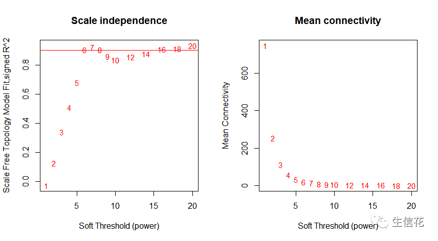
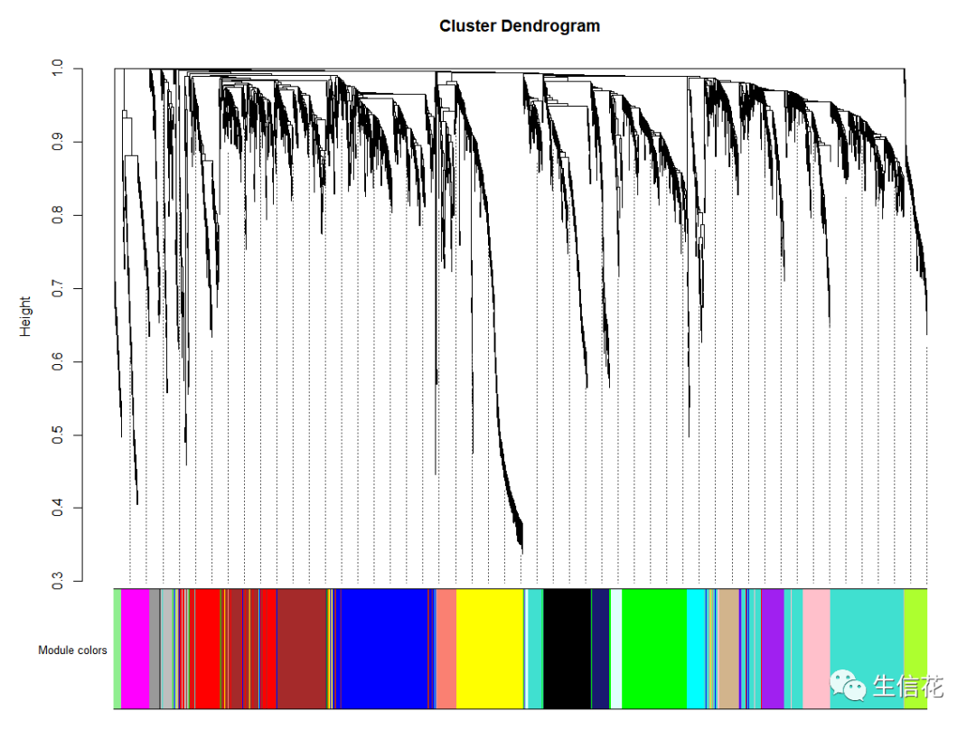
power = sft$powerEstimatesft$powerEstimate# 若无向网络在power小于15或有向网络power小于30内，没有一个power值使# 无标度网络图谱结构R^2达到0.8且平均连接度在100以下，可能是由于# 部分样品与其他样品差别太大。这可能由批次效应、样品异质性或实验条件对# 表达影响太大等造成。可以通过绘制样品聚类查看分组信息和有无异常样品。# 如果这确实是由有意义的生物变化引起的，也可以使用下面的经验power值。if(is.na(power)){# 官方推荐 "signed" 或 "signed hybrid"# 为与原文档一致，故未修改type = "unsigned"nSamples=nrow(datExpr)power = ifelse(nSamples<20, ifelse(type == "unsigned", 9, 18),ifelse(nSamples<30, ifelse(type == "unsigned", 8, 16),ifelse(nSamples<40, ifelse(type == "unsigned", 7, 14),ifelse(type == "unsigned", 6, 12))))}### 2.2一步法构建加权共表达网络，识别基因模块net = blockwiseModules(datExpr, power = power,TOMType = "unsigned", minModuleSize = 30,reassignThreshold = 0, mergeCutHeight = 0.25,numericLabels = TRUE, pamRespectsDendro = FALSE,saveTOMs = TRUE,saveTOMFileBase = "femaleMouseTOM",verbose = 3)### 2.4模块可视化，层级聚类树展示各个模块sizeGrWindow(12, 9)# Convert labels to colors for plottingmergedColors = labels2colors(net$colors)# Plot the dendrogram and the module colors underneathplotDendroAndColors(net$dendrograms[[1]], mergedColors[net$blockGenes[[1]]],"Module colors",dendroLabels = FALSE, hang = 0.03,addGuide = TRUE, guideHang = 0.05)

模块层级聚类树

### 2.5保存结果moduleLabels = net$colorsmoduleColors = labels2colors(net$colors)MEs = net$MEs;geneTree = net$dendrograms[[1]];save(MEs, moduleLabels, moduleColors, geneTree,file = "FemaleLiver-02-networkConstruction-auto.RData")

Step3 模块与外部临床特征都相关关系

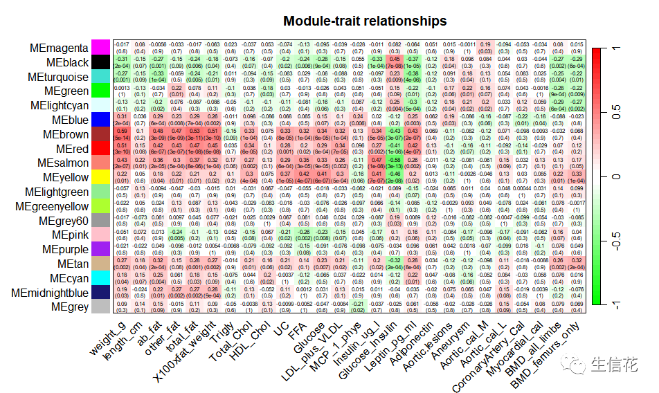
## 3.1数据准备load(file = "FemaleLiver-01-dataInput.RData");load(file = "FemaleLiver-02-networkConstruction-auto.RData");# Define numbers of genes and samplesnGenes = ncol(datExpr);nSamples = nrow(datExpr);# Recalculate MEs with color labelsMEs0 = moduleEigengenes(datExpr, moduleColors)$eigengenesMEs = orderMEs(MEs0)moduleTraitCor = cor(MEs, datTraits, use = "p");moduleTraitPvalue = corPvalueStudent(moduleTraitCor, nSamples);## 3.2模块与表型的相关性热图sizeGrWindow(10,6)# Will display correlations and their p-valuestextMatrix =  paste(signif(moduleTraitCor, 2), "n(",signif(moduleTraitPvalue, 1), ")", sep = "");dim(textMatrix) = dim(moduleTraitCor)par(mar = c(6, 8.5, 3, 3));# Display the correlation values within a heatmap plotlabeledHeatmap(Matrix = moduleTraitCor,xLabels = names(datTraits),yLabels = names(MEs),ySymbols = names(MEs),colorLabels = FALSE,colors = greenWhiteRed(50),textMatrix = textMatrix,setStdMargins = FALSE,cex.text = 0.5,zlim = c(-1,1),main = paste("Module-trait relationships"))

模块与表型的相关性热图

注：

# 请确保将路径”LiverFemale3600.csv”,”ClinicalTraits.csv”替换为实际数据集文件的路径，并根据需要调整模型参数和其他配置。

关于WGCNA分析，小花强烈推荐大家使用云生信平台（http://www.biocloudservice.com/home.html）进行WGCNA分析以及其他生信分析任务。云生信平台是一个强大而有趣的在线工具，为用户提供了简单、快速和可视化的生物信息学分析体验。

使用云生信平台，你可以轻松地上传和处理基因表达数据，进行WGCNA分析，并获得详细的结果和图表展示。你可以探索基因之间的共表达网络、发现关键模块、分析模块与临床特征的相关性等。同时，云生信平台还提供了许多其他生信分析工具和功能，如差异表达分析、功能富集分析、基因调控网络分析等，帮助你更全面地理解和解释你的数据。

使用云生信平台进行WGCNA分析不仅方便快捷，还能够节省大量的计算资源和时间。你可以随时随地访问平台，无需安装任何软件，直接在浏览器中进行分析。平台提供友好的用户界面和交互式操作，使得复杂的分析变得简单易懂。无论你是生物学研究者、生物信息学家还是学生，云生信平台都能满足你的分析需求，并帮助你探索数据背后的奥秘。所以，赶快来体验云生信平台吧！让生信分析变得更有趣、更高效！