用R进行GWAS分析,原来如此简单
点
击
蓝
字
★
关
注
我
们
使用R语言做GWAS分析,有些人对R语言可能比较熟悉,小师妹这里提供了一个用R语言分析GWAS的流程。该流程有:GWAS的QC,PCA分析,选择不同模型GWAS分析。
全基因组关联分析(Genome wide association study,GWAS)是对多个个体在全基因组范围的遗传变异(标记)多态性进行检测,获得基因型,进而将基因型与可观测的性状,即表型,进行群体水平的统计学分析,根据统计量或显著性P值筛选出最有可能影响该性状的遗传变异(标记),挖掘与性状变异相关的基因。
GWAS分析模型介绍
GWAS 分析一般会构建回归模型检验标记与表型之间是否存在关联。GWAS中的零假设(H0 null hypothesis)是标记的回归系数为零, 标记对表型没有影响。备择假设(H1,也叫对立假设,Alternative Hypothesis)是标记的回归系数不为零,SNP和表型相关。GWAS中的模型主要分为两种:
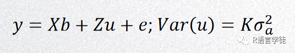
一般线性模型GLM(General Linear Model):y = Xβ + Zα + e
混合线性模型MLM(Mixed Linear Model):y = Xβ + Zα + Wμ+ e
y: 所要研究的表型性状;
Xβ:固定效应(Fixed Effect),影响y的其他因素,主要指群体结构;
Zα:标记效应(Marker Effect SNP);
Wμ:随机效应(RandomEffect),这里一般指个体的亲缘关系。
e: 残差
GWAS模型详细介绍
一般线性模型GLM:直接将基因型x和表型y做回归拟合。也可以加入群体结果控制假阳性。
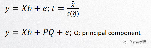
混合线性模型MLM:GLM模型中,如果两个表型差异很大,但群体本身还含有其他的遗传差异(如地域等),则那些与该表型无关的遗传差异也会影响到相关性。MLM模型可以把群体结构的影响设为协方差,把这种位点校正掉。此外,材料间的公共祖先关系也会导致非连锁相关,可加入亲缘关系矩阵作为随机效应来矫正。
FarmCPU:GWAS的瓶颈一是计算速度,二是统计准确性。FarmCPU能提升速度和准确性,首先把随机效应的亲缘关系矩阵(Kinship)转换为固定效应的关联SNP矩阵(S矩阵/QTNs矩阵),使计算速度大大加快;再利用QTN矩阵当做协变量,重新做关联分析,提升准确率。
话不多说直接上代码
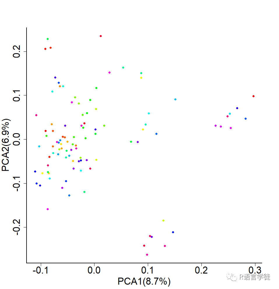
# get current working directorycur_wd<-getwd()# set path of working directorysetwd(cur_wd)# quality control for gene chipsystem('plink --cow --file 1-data-holstein --mind 0.1 --geno 0.1 --maf 0.05 --hwe 0.00001 --recode --out 2-data-holstein_qc')system('plink --cow --file 1-data-holstein --mind 0.1 --geno 0.1 --maf 0.05 --hwe 0.00001 --make-bed --out 2-data-holstein_qc')system('plink --cow --file 1-data-holstein --mind 0.1 --geno 0.1 --maf 0.05 --hwe 0.00001 --recodeA --out 2-data-holstein_qc')#PCAsystem('plink --cow --bfile 2-data-holstein_qc --pca 20 --out 2-data-holstein_pca')# plot for PCA# import data of eigenvectors and eigenvaluespca_eigenvectors<-read.table('2-data-holstein_pca.eigenvec')pca_eigenval<-read.table('2-data-holstein_pca.eigenval')#calculating percentage of eigenvaluespca_eigenval$percentage<-pca_eigenval$V1/sum(pca_eigenval$V1)#plotpca_value1<-paste("PCA1(",100*round(pca_eigenval$percentage[1],3),"%)",sep = "")pca_value2<-paste("PCA2(",100*round(pca_eigenval$percentage[2],3),"%)",sep = "")# output plottiff("2-plot-PCA.tiff", width = 1000,height=1000,res = 100)par(mar=c(5,5,5,5),cex.axis=2,cex.lab=2, cex.axis=2, lwd=2 ,bty="l")plot(pca_eigenvectors[,c(3,4)],pch=16,col=rainbow(100),xlab=pca_value1,ylab=pca_value2)dev.off()
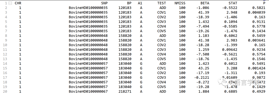
# export eigenvectors as covariatewrite.table(pca_eigenvectors[,1:7],"2-data-covariate_pca.txt",row.names = F,col.names = F,quote = F)# t testsystem("plink --cow --bfile 2-data-holstein_qc --pheno 1-data-phenotype.txt --mpheno 1 --linear --out 3-result-1-ttest")# glmsystem("plink --cow --bfile 2-data-holstein_qc --pheno 1-data-phenotype.txt --mpheno 1 --covar 2-data-covariate_pca.txt --covar-number 1-5 --linear --out 3-result-2-glm")# mlmsystem("gcta64 --autosome-num 30 --bfile 2-data-holstein_qc --pheno 1-data-phenotype.txt --mpheno 1 --mlma --out 3-result-3-mlm")# mlm Q+Ksystem("gcta64 --autosome-num 30 --bfile 2-data-holstein_qc --pheno 1-data-phenotype.txt --mpheno 1 --qcovar 2-data-covariate_pca.txt --mlma --out 3-result-4-mlm")#FarmCPUinstall.packages("bigmemory")install.packages("biganalytics")library(bigmemory)library(biganalytics)library(compiler)source('1-farmcpu.txt')source('1-gapit.txt')#import phenotype dataphenotype<-read.table("1-data-phenotype.txt",header = F)phenotype<-phenotype[,-1]names(phenotype)<-c("id","yield","fat")#import map for genotype(3 column):SNPChromosomePositiongenotype_map<-read.table("2-data-holstein_qc.map",header = F)genotype_map<-genotype_map[,c(2,1,4)]names(genotype_map)<-c("SNP","Chromosome","Position")#import genotype:ID+genotype(numeric:0 1 2),titile=T:ID+snp_namegenotype<-read.big.matrix("2-data-holstein_qc.raw",type="char",sep = " ",head = TRUE)genotype<-genotype[,-c(1,3:6)]#set the threshold for first iteration step#first_thero=max(0.05/table(genotype_map[,2]))myFarmCPU<-FarmCPU(Y=phenotype[,c(1,2)],GD=genotype,GM=genotype_map,p.threshold = first_thero,cutOff = 0.05,MAF.calculate = F,threshold.output = 1,#method.bin = "optimum",DPP=10000)# import results# t testresult_ttest<-read.table("3-result-1-ttest.assoc.linear",header = T)
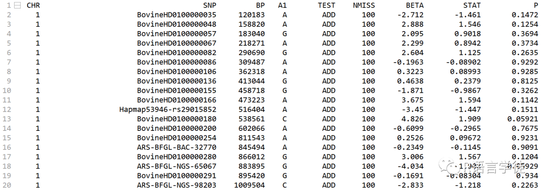
# glmresult_glm<-read.table("3-result-2-glm.assoc.linear",header = T)result_glm<-result_glm[which(result_glm$TEST=="ADD"),]
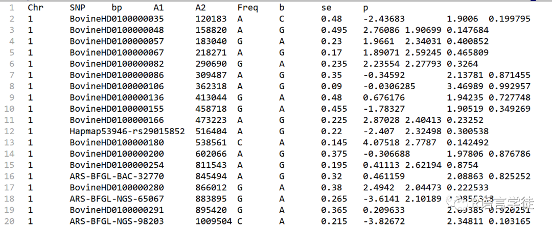
#mlmresult_mlm<-read.table("3-result-3-mlm.mlma",header = T)
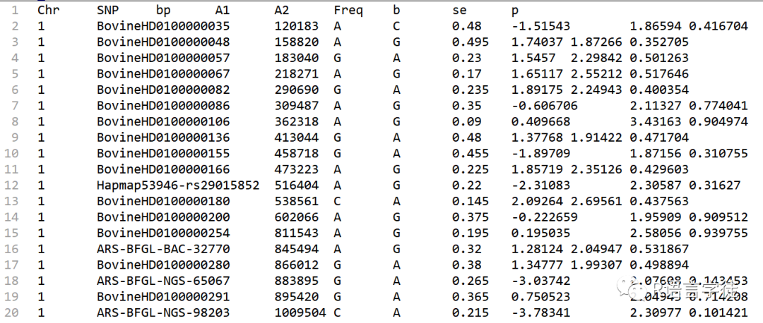
#mlm Q+Kresult_mlm_q<-read.table("3-result-4-mlm.mlma",header = T))
# farmcpuresult_farmcpu<-read.csv(paste("FarmCPU",names(phenotype)[2],"GWAS","Results.csv",sep = "."),header = T)
学完了操作流程是不是想马上操作一番,小师妹也在资料中存放了测试数据“1-data-holstein.map”,“1-data-holstein.ped”以及操作视频讲解。加师妹微信获取资料哦~大家可以学习并测试一下,让知识更加牢固。
小伙伴们也可以用我们的工具云生信平台在线分析。
网址: http://www.biocloudservice.com/home.html
★

名额有限,赶快扫码联系小师妹吧!