高分生信SCI-WGCNA分析复现
生信人R语言学习必备
立刻拥有一个Rstudio账号
开启升级模式吧
(56线程,256G内存,个人存储1T)

今天小果给小伙伴带来的分享是啥呢?
今天小果将复现一篇8+生信文章中的WGCNA分析,通过该推文将掌握如何利用自己的数据进行WGCNA分析,来进行与表型或者疾病相关候选基因的挖掘,小果觉得WGCNA是一个非常不错的候选基因挖掘的方法,值得小伙伴们认真学习,接下来跟着小果开始今天的分享吧!
1.WGCNA介绍
在开始分析之前,小果想为小伙伴简单介绍一下WGCNA,WGCNA是一种用于基因共表达的方法,它可以将高通量基因表达数据转化为一个共表达网络,从而发现具有相似表达模式的基因模块,以及研究这些模块与表型之间的相关性,最终挖掘与表型相关的候选基因。这就是小果对WGCNA分析原理的简单介绍,是不是通俗易懂奥!其实WGCNA分析很简单,小伙伴不要因为分析步骤多而不敢尝试,只需要输入基因表达矩阵和对应样本表型数据文件,就可以完成分析,有需要的小伙伴可以跟着小果开始今天的实操。
2.准备需要的R包
#安装需要的R包
BiocManager::install("WGCNA")#加载需要的R包
library(WGCNA)3.WGCNA分析
#读取表达矩阵,行名为基因,列名为样本信息
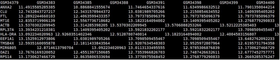
expr<-read.table(“combined.expr.txt”,header=T,sep=”t”)
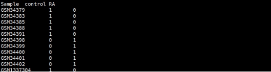
#行列转置mydata<-exprexpr2<-data.frame(t(mydata))#确定expr2列名colnames(expr2)<-rownames(mydata)#确定expr2行名rownames(expr2)<-colnames(mydata)#基因过滤dataExpr1<-expr2gsg=goodSamplesGenes(dataExpr1,verbose=3);gsg$allOKif (!gsg$allOK){# Optionally, print the gene and sample names that were removed:if (sum(!gsg$goodGenes)>0)printFlush(paste("Removing genes:",paste(names(dataExpr)[!gsg$goodGenes], collapse = ",")));if (sum(!gsg$goodSamples)>0)printFlush(paste("Removing samples:",paste(rownames(dataExpr)[!gsg$goodSamples], collapse = ",")));# Remove the offending genes and samples from the data:dataExpr1 = dataExpr1[gsg$goodSamples, gsg$goodGenes]}#基因数目nGenes = ncol(dataExpr1)#样本数目nSamples = nrow(dataExpr1)#导入表型数据,第一列为样本信息,其他列为表型数据,需要注意的是表型数据要与样本数据一一对应traitData=read.table("TraitData.txt",header=T,sep="t",row.names=1)
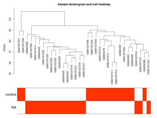
#提取表达矩阵样本名fpkmSamples<-rownames(dataExpr1)#提取表型文件样本名traitSamples<-rownames(traitData)#表达矩阵样本名顺序匹配表型文件样本名traitRows<-match(fpkmSamples,traitSamples)#获得匹配好样本顺序的表型文件dataTraits<-traitData[traitRows,]#绘制树+表型热图sampleTree2<-hclust(dist(dataExpr1),method="average")traitColors<-numbers2colors(dataTraits,signed=FALSE)png("sample-subtype-cluster.png",width = 800,height = 600)plotDendroAndColors(sampleTree2,traitColors,groupLabels=names(dataTraits),main="Sample dendrogram and trait heatmap",cex.colorLabels=1.5,cex.dendroLabels=1,cex.rowText=2)dev.off()
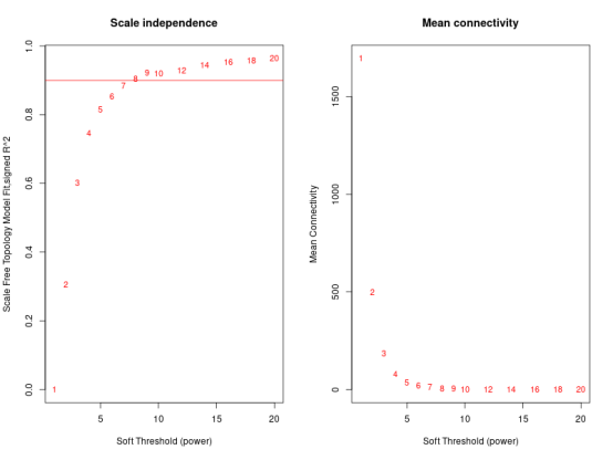
#计算合适的power值,并绘制Power值曲线图powers = c(c(1:10), seq(from = 12, to=20, by=2))sft = pickSoftThreshold(dataExpr1, powerVector = powers, verbose = 5)#设置网络构建参数选择范围,计算无尺度分布拓扑矩阵png("step2-beta-value.png",width = 800,height = 600)par(mfrow = c(1,2));cex1 = 0.9;# Scale-free topology fit index as a function of the soft-thresholding powerplot(sft$fitIndices[,1], -sign(sft$fitIndices[,3])*sft$fitIndices[,2],xlab="Soft Threshold (power)",ylab="Scale Free Topology Model Fit,signed R^2",type="n",main = paste("Scale independence"));text(sft$fitIndices[,1], -sign(sft$fitIndices[,3])*sft$fitIndices[,2],labels=powers,cex=cex1,col="red");abline(h=0.90,col="red")# Mean connectivity as a function of the soft-thresholding powerplot(sft$fitIndices[,1], sft$fitIndices[,5],xlab="Soft Threshold (power)",ylab="Mean Connectivity", type="n",main = paste("Mean connectivity"))text(sft$fitIndices[,1], sft$fitIndices[,5], labels=powers, cex=cex1,col="red")dev.off()
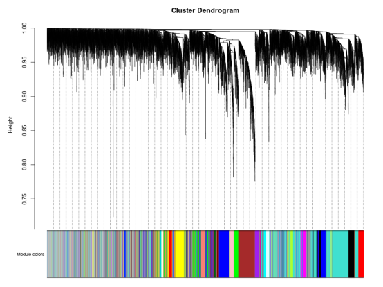
#一步法构建共表达网络##需要调用WGCNA包自带的cor函数,不然会发生报错奥!cor<-WGCNA::cor##在进行共表达网络构建时,power值的选择非常重要,最影响结果的一个参数,需要经过多次尝试,才能找到最适合的。net = blockwiseModules(dataExpr1, power = 7, maxBlockSize = nGenes,TOMType ='unsigned', minModuleSize = 30,reassignThreshold = 0, mergeCutHeight = 0.25,numericLabels = TRUE, pamRespectsDendro = FALSE,saveTOMs=TRUE, saveTOMFileBase = "drought",verbose = 3)table(net$colors)cor<-stats::cor#绘制基因聚类树和模块颜色组合# Convert labels to colors for plottingmoduleLabels = net$colorsmoduleColors = labels2colors(moduleLabels)# Plot the dendrogram and the module colors underneathpng("step4-genes-modules.png",width = 800,height = 600)plotDendroAndColors(net$dendrograms[[1]], moduleColors[net$blockGenes[[1]]],"Module colors",dendroLabels = FALSE, hang = 0.03,addGuide = TRUE, guideHang = 0.05)dev.off()
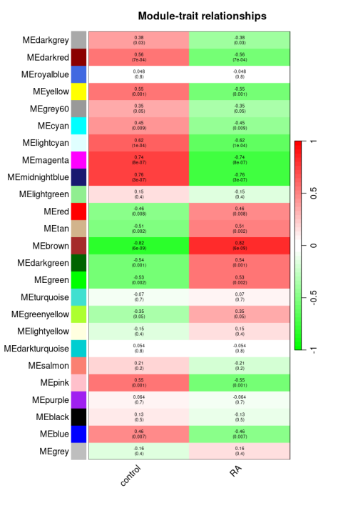
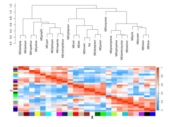
#计算模块与性状间的相关性及绘制相关性热图nGenes = ncol(dataExpr1)nSamples = nrow(dataExpr1)design=read.table("TraitData.txt", sep = 't', header = T, row.names = 1)# Recalculate MEs with color labelsMEs0 = moduleEigengenes(dataExpr1, moduleColors)$eigengenes##不同颜色的模块的ME值矩 (样本vs模块)MEs = orderMEs(MEs0);moduleTraitCor = cor(MEs, design , use = "p");moduleTraitPvalue = corPvalueStudent(moduleTraitCor, nSamples)# Will display correlations and their p-valuestextMatrix = paste(signif(moduleTraitCor, 2), "n(",signif(moduleTraitPvalue, 1), ")", sep = "");dim(textMatrix) = dim(moduleTraitCor)png("step5-Module-trait-relationships.png",width = 800,height = 1200,res = 120)par(mar = c(6, 8.5, 3, 3));# Display the correlation values within a heatmap plotlabeledHeatmap(Matrix = moduleTraitCor,xLabels = colnames(design),yLabels = names(MEs),ySymbols = names(MEs),colorLabels = FALSE,colors = greenWhiteRed(50),textMatrix = textMatrix,setStdMargins = FALSE,cex.text = 0.5,zlim = c(-1,1),main = paste("Module-trait relationships"))dev.off()
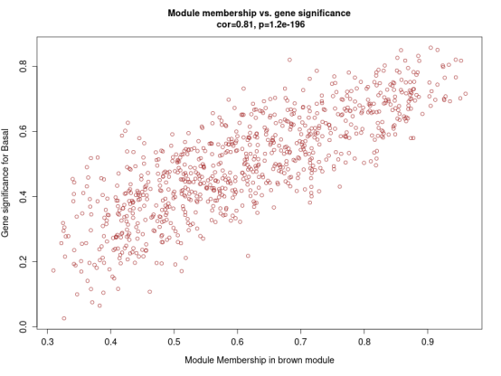
#计算MM值和GS值并绘图##切割,从第三个字符开始保存modNames = substring(names(MEs), 3)geneModuleMembership = as.data.frame(cor(dataExpr1, MEs, use = "p"));## 算出每个模块跟基因的皮尔森相关系数矩## MEs是每个模块在每个样本里面皿## dataExpr1是每个基因在每个样本的表达量MMPvalue = as.data.frame(corPvalueStudent(as.matrix(geneModuleMembership), nSamples) ##计算MM值对应的P值);names(geneModuleMembership) = paste("MM", modNames, sep=""); ##给MM对象统一赋名names(MMPvalue) = paste("p.MM", modNames, sep=""); ##给MMPvalue对象统一赋名##计算基因与每个性状的显著性(相关性)及pvalue值geneTraitSignificance = as.data.frame(cor(dataExpr1, design, use = "p"));GSPvalue = as.data.frame(corPvalueStudent(as.matrix(geneTraitSignificance), nSamples) ##计算GS值对应的pvalue值);names(geneTraitSignificance) = paste("GS.", colnames(design), sep="");names(GSPvalue) = paste("p.GS.", colnames(design), sep="");module = "brown"column = match(module, modNames); ##在所有模块中匹配选择的模块,返回所在的位置moduleGenes = moduleColors==module; ##==匹配,匹配上的返回True,否则返回falsepng("step6-Module_membership-gene_significance.png",width = 800,height = 600)par(mfrow = c(1,1)); ##设定输出图片行列数量,(1_1)代表行一个,列一丿verboseScatterplot(abs(geneModuleMembership[moduleGenes, column]), ## 绘制MM和GS散点囿abs(geneTraitSignificance[moduleGenes, 1]),xlab = paste("Module Membership in", module, "module"),ylab = "Gene significance for Basal",main = paste("Module membership vs. gene significancen"),cex.main = 1.2, cex.lab = 1.2, cex.axis = 1.2, col = module)dev.off()
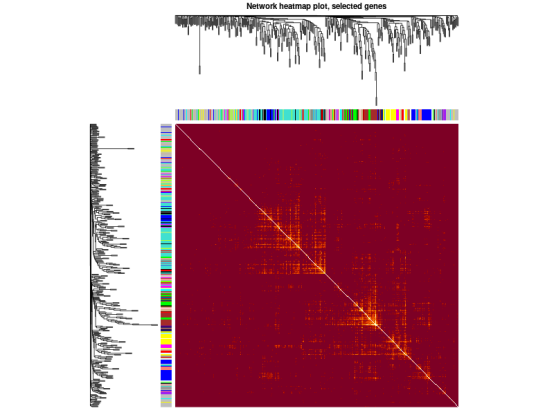
#绘制TOM热图+模块性状组合图geneTree = net$dendrograms[[1]]; ##提取基因聚类dissTOM = 1-TOMsimilarityFromExpr(dataExpr1, power = 7); ##计算TOM距离plotTOM = dissTOM^7; ##通过7次方处理进行标准化,降低基因间的误差diag(plotTOM) = NA; ##替换斜对角矩阵中的内容为NATOMplot(plotTOM, geneTree, moduleColors, main = "Network heatmap plot, all genes")nSelect = 400 ##挑选需要提取的基因set.seed(10); ##设置随机种子数,保证选取的随机性select = sample(nGenes, size = nSelect); ##仿5000个基因中随机叿400丿selectTOM = dissTOM[select, select]; ##提取挑出来的基因的TOM距离# There’s no simple way of restricting a clustering tree to a subset of genes, so we must re-cluster.selectTree = hclust(as.dist(selectTOM), method = "average") ##对挑出来对基因TOM距离重新聚类selectColors = moduleColors[select];# Open a graphical windowsizeGrWindow(9,9)# Taking the dissimilarity to a power, say 10, makes the plot more informative by effectively changingplotDiss = selectTOM^7; ##对挑选出对基因TOM距离7次方处理diag(plotDiss) = NA; ##替换斜对角矩阵中的内容为NApng("step7-Network-heatmap.png",width = 800,height = 600)TOMplot(plotDiss, selectTree, selectColors, ##绘制TOM图main = "Network heatmap plot, selected genes")dev.off()
# 模块性状组合图RA = as.data.frame(design[,2]); ##提取特定性状names(RA) = "RA"# Add the weight to existing module eigengenesMET = orderMEs(cbind(MEs, RA))# Plot the relationships among the eigengenes and the traitsizeGrWindow(5,7.5);par(cex = 0.9)png("step7-Eigengene-dendrogram.png",width = 800,height = 600)plotEigengeneNetworks(MET, "", ##绘制模块聚类图和热图marDendro =c(0,5,1,5), ##树类图区间大小谁宿marHeatmap = c(5,6,1,2), cex.lab = 0.8, ##树类图区间大小谁宿xLabelsAngle = 90) ##轴鲜艿90庿dev.off()
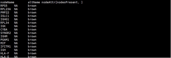
#导出单个模块的网络结果TOM = TOMsimilarityFromExpr(dataExpr1, power = 7); ##需要较长时间# 选择brown模块module = "brown";# Select module probesprobes = colnames(dataExpr1)inModule = (moduleColors==module);## 提取指定模块的基因名modProbes = probes[inModule];

modTOM = TOM[inModule, inModule];dimnames(modTOM) = list(modProbes, modProbes)## 模块对应的基因关系矩cyt = exportNetworkToCytoscape( ##导出单个模块的Cytoscape输入文件modTOM,edgeFile = paste("CytoscapeInput-edges-", paste(module, collapse="-"), ".txt", sep=""), ##输出边文件名nodeFile = paste("CytoscapeInput-nodes-", paste(module, collapse="-"), ".txt", sep=""), ##输出点文件名weighted = TRUE,threshold = 0.02,nodeNames = modProbes,nodeAttr = moduleColors[inModule])
CytoscapeInput-edges-brown.txt,边文件
CytoscapeInput-nodes-brown.txt,点文件
最终小果成功完成了WGCNA分析,基本达到了复现,今天小果的分享就到这里啦!如果小伙伴有其他数据分析需求,可以尝试本公司新开发的生信分析小工具云平台,零代码完成分析,非常方便奥,云平台网址为:http://www.biocloudservice.com/home.html,包括了WGCNA分析(http://www.biocloudservice.com/336/336.php),GEO数据下载(http://www.biocloudservice.com/371/371.php)等小工具,欢迎大家和小果一起讨论学习哈!!!!

点击“阅读原文”立刻拥有
↓↓↓