生信文章必备分析内容,对亚型利用MCPcounter和CIBERSORT两种算法进行免疫浸润分析
点击蓝字 关注我们
今天小花带来的分享为首先利用ConsensusCluster对肿瘤样本进行分型,然后对不同亚型利用MCPcounter和CIBERSORT两种算法进行免疫浸润分析,最后对不同亚型之间免疫细胞类型进行显著差异分析,该分析在生信文章中出现的频率非常高,值得小伙伴们学习嗷,接下来跟着小花开启今天的学习之旅吧!
准备需要的R包
#安装需要的R包install.packages("tidyverse")install.packages("devtools")library(devtools)install_github("ebecht/MCPcounter",ref="master", subdir="Source")install.packages("ggplot2")install.packages("ggsci")BiocManager::install("ConsensusClusterPlus")#加载需要的R包library(MCPcounter)library(reshape2)library(ggpubr)library(ggplot2)library(tidyverse)library(ggsci)library(ConsensusClusterPlus)source('Cibersort.R')
ConsensusCluster一致性聚类分析
#筛选出的有预后的TEX基因表达矩阵文件,行名为基因名,列为样本名expr1<- read.table(file = "expr_cluster.txt",#工作目录下的文件名header = T,#设置有列名sep = "t",#分隔符row.names = 1,#设置行名check.names=F)#不检查行名dir.create('ConsensusCluster/')#构建文件夹#ConsensusCluster一致性聚类results = ConsensusClusterPlus(as.matrix(expr1),maxK=6,reps=100,pItem=0.8,pFeature=1,title='ConsensusCluster/',clusterAlg="km",distance="euclidean",seed=123456,plot="pdf")icl <- calcICL(results,title = 'ConsensusCluster/',plot = 'pdf')Kvec = 2:6x1 = 0.1; x2 = 0.6PAC = rep(NA,length(Kvec))names(PAC) = paste("K=",Kvec,sep="")for(i in Kvec){M = results[[i]]$consensusMatrixFn = ecdf(M[lower.tri(M)])PAC[i-1] = Fn(x2) - Fn(x1)}optK = Kvec[which.min(PAC)]optKPAC <- as.data.frame(PAC)PAC$K <- 2:6#绘制PAC验证曲线ggplot(PAC,aes(factor(K),PAC,group=1))+geom_line()+theme_bw()+theme(panel.grid = element_blank())+geom_point(size=4,shape=21,color='darkred',fill='skyblue')+ylab('Proportion of ambiguous clustering')+xlab('Cluster number K')ggsave("PAC.pdf")#最小值也就是最佳K,仍然为3.#提取分型信息,k=3clusterNum=3 #k值变化调整cluster=results[[clusterNum]][["consensusClass"]]sub <- data.frame(Sample=names(cluster),Cluster=cluster)sub$Cluster <- paste0('C',sub$Cluster)table(sub$Cluster)write.table(sub,file = "K3.txt",sep="t",quote=F)#输出结果
亚型间利用MCPCounter算法进行免疫浸润显著差异分析
#EXP.txt,基因表达矩阵文件,行名为基因名,列名为样本信息。exp<-read.table("EXP.txt",header=T,row.names=1,sep="t",check.names=F)
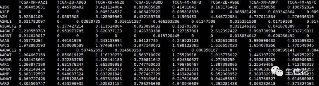
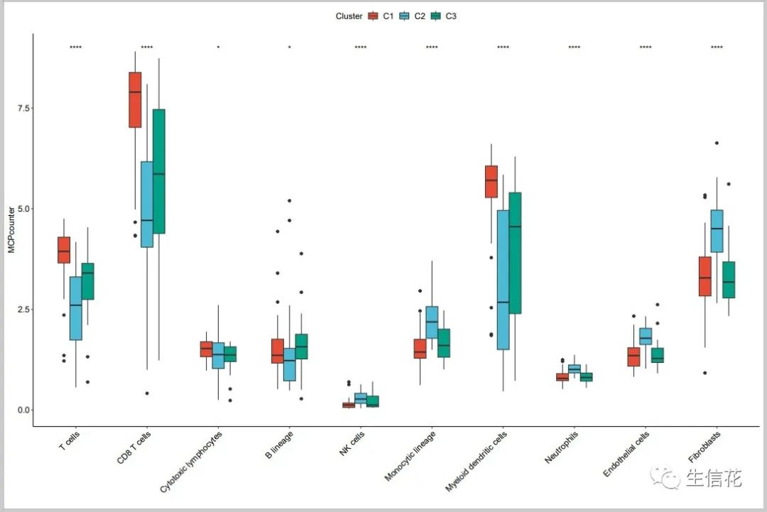
#利用MCPcount R包计算免疫浸润丰度,通过MCPcounter.estimate函数进行计算MCP<- MCPcounter.estimate(exp, featuresType = "HUGO_symbols")#保存MCPcounter结果文件write.table(MCP,file="MCPcounter.txt",row.names=T,col.names=T,quote=F,sep="t")#行列转置MCP<-as.data.frame(t(MCP))#将行名转化为列名MCP<-rownames_to_column(MCP,var="Sample")#连接亚型分组信息和免疫细胞MCPcluster<-left_join(MCP,sub,by="Sample")#长宽数据转换MCPcluster<-melt(MCPcluster,id.vars=c("Sample","Cluster"))#设置列名colnames(MCPcluster)<-c("Sample","Cluster","celltype","MCPcounter")#绘制显著差异分析小提琴+箱线图boxplot_MCPCounter<- ggplot(MCPcluster, aes(x = celltype, y = MCPcounter))+labs(y="MCPcounter",x= "")+geom_boxplot(aes(fill = Cluster),position=position_dodge(0.5),width=0.5)+scale_fill_npg()+#修改主题theme_classic() +theme(axis.title = element_text(size = 12,color ="black"),axis.text = element_text(size= 12,color = "black"),panel.grid.minor.y = element_blank(),panel.grid.minor.x = element_blank(),axis.text.x = element_text(angle = 45, hjust = 1 ),panel.grid=element_blank(),legend.position = "top",legend.text = element_text(size= 12),legend.title= element_text(size= 12)) +stat_compare_means(aes(group = Cluster),label = "p.signif",method = "kruskal.test",#kruskal.test多组检验hide.ns = T)#隐藏不显著的ggsave(file="MCPCounter.pdf",boxplot_MCPCounter,height=10,width=15)
CIBERSORT算法中不同亚型之间免疫浸润显著差异分析
#22种免疫细胞表达量文件,第一列为Gene symbol,其他列为22种免疫细胞LM22.file <- "LM22.txt"
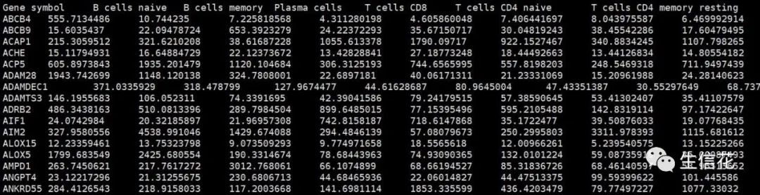
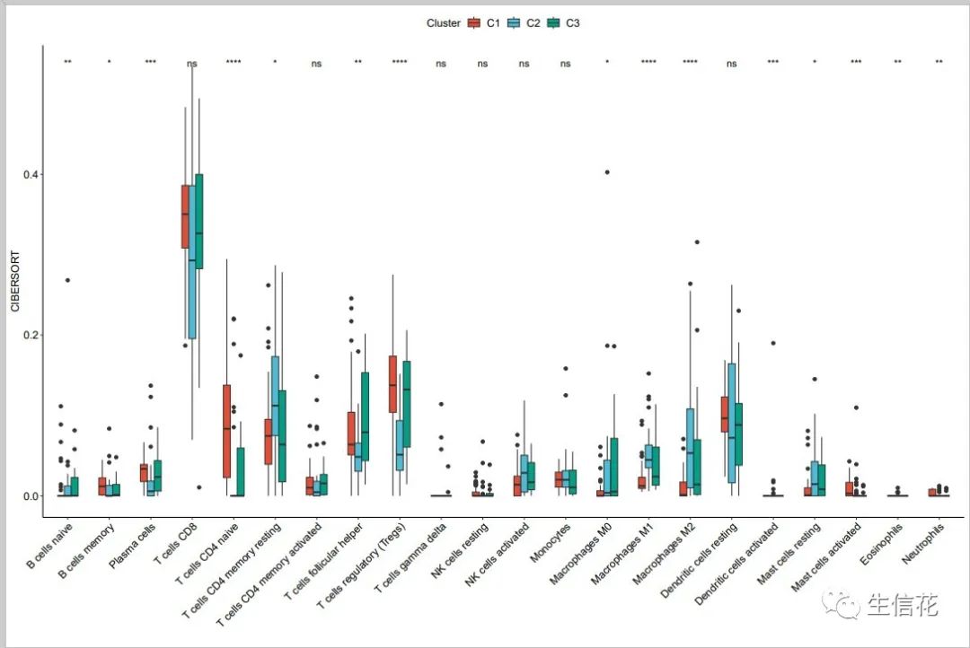
#基因表达矩阵文件TCGA_exp.file <- "EXP.txt"#perm表示置换次数, QN如果是芯片设置为T,如果是测序就设置为FTCGA_cibersort.results <- CIBERSORT(LM22.file ,TCGA_exp.file, perm = 50, QN = F)write.table(TCGA_cibersort.results, "TCGA_CIBERSORT.txt",sep="t",col.names=T,row.names=T,quote=F)# 提取cibersort前22列数据,23-25列为 P-value, P-value,RMSE数据cibersort_data <- as.data.frame(TCGA_cibersort.results[,1:22])#将行名转化为列名cibersort_data<-rownames_to_column(cibersort_data,var="Sample")#连接亚型分组信息和免疫细胞cibersort<-left_join(cibersort_data,sub,by="Sample")#长宽数据转换cibersort<-melt(cibersort,id.vars=c("Sample","Cluster"))#设置列名colnames(cibersort)<-c("Sample","Cluster","celltype","CIBERSORT")#绘制显著差异小提琴+箱线图boxplot_CIBERSORT<- ggplot(cibersort, aes(x = celltype, y =CIBERSORT ))+labs(y="CIBERSORT",x= "")+geom_boxplot(aes(fill = Cluster),position=position_dodge(0.5),width=0.5)+scale_fill_npg()+#修改主题theme_classic() +theme(axis.title = element_text(size = 12,color ="black"),axis.text = element_text(size= 12,color = "black"),panel.grid.minor.y = element_blank(),panel.grid.minor.x = element_blank(),axis.text.x = element_text(angle = 45, hjust = 1 ),panel.grid=element_blank(),legend.position = "top",legend.text = element_text(size= 12),legend.title= element_text(size= 12)) +stat_compare_means(aes(group = Cluster),label = "p.signif",#添加星号标签method = "kruskal.test",#kruskal.test多组检验hide.ns = F)#显示不显著的#保存图片ggsave(file="CIBERSORT.pdf",boxplot_CIBERSORT,height=10,width=15)
结果文件
1.MCPCounter.pdf
该结果图片为 MCPCounter算法中不同亚型之间具有显著差异的免疫细胞类型比较图,1表示p小于0.05,11表示p小于0.01,111表示p小于0.001
2.CIBERSORT.pdf
该结果图片为 CIBERSORT算法中不同亚型之间具有显著差异的免疫细胞类型比较图,1表示p小于0.05,11表示p小于0.01,111表示p小于0.001
3.MCPcounter.txt
该结果文件为利用MCPcounter算法计算的免疫细胞矩阵,行名为免疫细胞类型,列名为样本名。

4.TCGA_CIBERSORT.txt
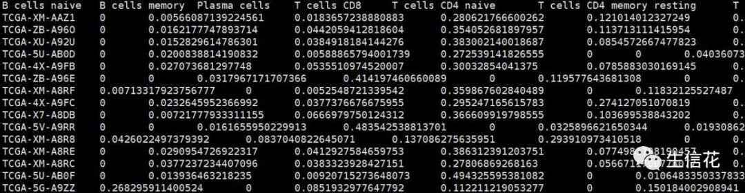
该结果文件为利用CIBERSORT算法计算的免疫细胞矩阵,列名为免疫细胞类型,行名为样本名。
5.K3.txt
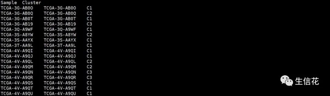
该结果文件为利用ConsensusCluster一致性聚类分析,K=3时亚型分组信息文件,第一列为样本名,第二列为分组信息。
最终小花成功的对不同亚型通过CIBERSORT和MCPcounter算法进行了免疫浸润分析,,看起来图片效果非常不错,欢迎大家和小花一起讨论学习呀!免疫浸润相关分析内容,例如单样本富集算法分析免疫浸润丰度(http://www.biocloudservice.com/106/106.php),计算64种免疫细胞相对含量(http://www.biocloudservice.com/107/107.php)等都可以用本公司新开发的零代码云平台生信分析小工具,一键完成该分析嗷,感兴趣的小伙伴欢迎来尝试奥,网址:http://www.biocloudservice.com/home.html。今天小花的分享就到这里,下期再见奥。
欢迎使用:云生信 – 学生物信息学 (biocloudservice.com)
如果想用服务器可以联系微信:18502195490(快来联系我们使用吧!)


(点击阅读原文跳转)
![]() 点一下阅读原文了解更多资讯
点一下阅读原文了解更多资讯