怎样迈出精准医学分析第一步?Xeva帮你打好药物靶向的基础!

领取本篇代码、基因集或示例数据等文件
文件编号:240118
需要租赁服务器的小伙伴可以扫码添加小果,此外小果还提供生信分析,思路设计,文献复现等,有需要的小伙伴欢迎来撩~

 |
#检查和安装Xevalibrary(devtools)if(is.element("Xeva", installed.packages())==FALSE){ install_github("bhklab/Xeva")} library(Xeva)
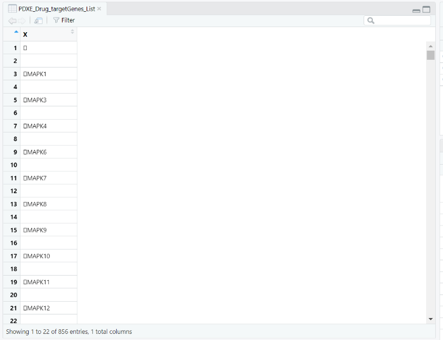
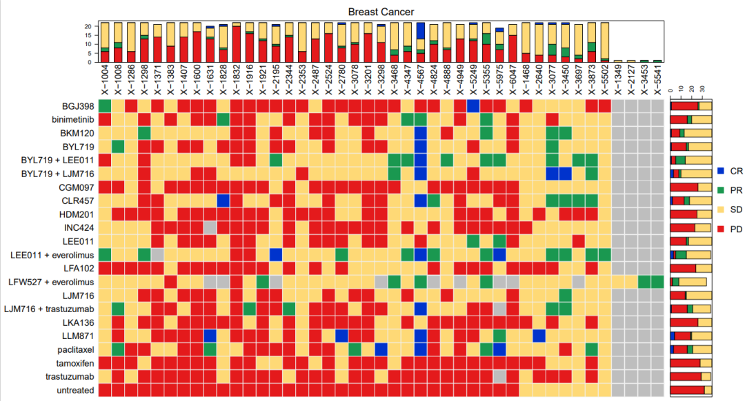
#安装所需R包library(methods)library(BBmisc)library(Xeva)#加载患者的肿瘤反应数据data(pdxe)#将肿瘤的缩写和全称对应,方便绘图tumor <- c("BRCA" = "Breast Cancer","NSCLC" = "Non-small Cell Lung Carcinoma","PDAC" = "Pancreatic Ductal Carcinoma","CM" = "Cutaneous Melanoma","GC" = "Gastric Cancer","CRC" = "Colorectal Cancer")#输出PDF文件,根据Xeva中的mRECIST 标准,按照患者的ID和肿瘤类型进行了分组,得到了一个新的数据集 pdxe.ttpdf("../results/figure-1.pdf", width = 14.1, height = 7.6)for(tt in names(tumor)){ pdxe.tt <- summarizeResponse(pdxe, response.measure = "mRECIST",group.by="patient.id", tissue=tt) pdxe.tt <- pdxe.tt[, names(sort(pdxe.tt["untreated", ], na.last = TRUE))] plotmRECIST(pdxe.tt, control.name = "Untreated", name = tumor[tt], row_fontsize = 12, col_fontsize=12, sort = FALSE)}dev.off()
#导入功能函数,所用包set.seed(19)#调用功能函数文件source("imp_functions.R")suppressMessages(library(Biobase))library(Rtsne)library(ggplot2)library(ggpubr)
#准备输出结果args <- commandArgs(trailingOnly = TRUE)recompute <- FALSEif(args[1] %in% c(TRUE, FALSE)){ recompute <- args[1] }
pdf("../results/figure-2.pdf", width = 9.27, height = 6.4)
#从"../data/passage_data.Rda"文件中读取通道数据。passage <- readRDS("../data/passage_data.Rda")dp <- pData(passage$data)
#对数据进行t-SNE(t分布随机邻居嵌入)降维处理#计算肿瘤对应的患者数量,排序ptByTT <- sort(sapply(unique(dp$tumor.type),function(tt){length(unique(dp[dp$tumor.type==tt, "patient.id"]))}, USE.NAMES = TRUE))#筛选数量大于10的肿瘤类型tt2take <- names(ptByTT)[ptByTT>10]dq <- dp[dp$tumor.type %in% tt2take, ]psgFrq<- table(dq$patient.id)pid2take <- names(psgFrq)[psgFrq>1]dq <- dq[dq$patient.id%in%pid2take, ]dq$tumor.type <- gsub("_", " ", dq$tumor.type)dq$tumor.type[dq$tumor.type=="large intestine"] <- "LI"
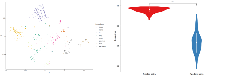
tissuCol <- c('#1b9e77','#d95f02','#7570b3','#e7298a', '#d9f0a3', '#e6ab02','#a6761d','#666666')names(tissuCol) <- c("lung", "ovary", "LI", "breast", "kidney", "pancreas","skin", "soft tissue") #筛选数据dt <- as.matrix(t(Biobase::exprs(passage$data)))dt <- dt[dq$biobase.id, ]#运行t-SNE算法分析tsne_out <- Rtsne(dt, perplexity = 13)dq$X <- data.frame(tsne_out$Y)[,1]dq$Y <- data.frame(tsne_out$Y)[,2]#进行可视化分析tsne.plot <- ggplot(data=dq, aes(X, Y, color=tumor.type)) + geom_point(size=0.5)tsne.plot <- tsne.plot + theme_classic()tsne.plot <- tsne.plot + scale_color_manual(values=tissuCol)tsne.plot <- tsne.plot + geom_line(data=dq, aes(X, Y, group=patient.id), show.legend=FALSE)print(tsne.plot)
#对肿瘤数据的相关性进行分析marExp <- Biobase::exprs(passage$data)passMat <- passage$passage
# 过滤有多个非 NA 值的行和列passMat <- passMat %>% filter(rowSums(!is.na(.)) > 1) %>% filter(colSums(!is.na(.)) > 1)
if(recompute==TRUE){ cat(sprintf("recomputing values.... it may take long timen")) dfx <- data.frame()##----- correlation for related pairs ------------# use map_dfr to loop over the rows and return a data frame dfx <- passMat %>% map_dfr(~{# use combn to get all possible pairs of non-NA values prx <- combn(.x[!is.na(.x)], 2, simplify = F)# use map_dbl to loop over the pairs and return a numeric vector v <- prx %>% map_dbl(~cor(marExp[, .x[1]], marExp[, .x[2]], method = "pearson"))# return a data frame with correlation and type data.frame(Correlation = v, type = "Related pairs") })
# 使用 sample_n 获取行的随机样本 randPassMat <- passMat %>% sample_n(nrow(passMat))
# 使用 map_dfr 遍历行并返回数据帧 dfx <- randPassMat %>% map_dfr(~{# use combn to get all possible pairs of non-NA values prx <- combn(.x[!is.na(.x)], 2, simplify = F)# use keep to filter the pairs that are not in the same row of passMat prx <- prx %>%keep(~!any(passMat[which(passMat == .x[1]), ] == .x[2]))#使用 map_dbl 遍历这些对并返回一个数值向量 v <- prx %>% map_dbl(~cor(marExp[, .x[1]], marExp[, .x[2]]))# return a data frame with correlation and type data.frame(Correlation = v, type = "Random pairs") })} else{ cat(sprintf("using pre-computed valuesn")) dfx <- readRDS("../data/PDX_passage_correlation.Rda")}
pltOrd <- c("Related pairs", "Random pairs")dfx$type <- factor(as.character(dfx$type), levels = pltOrd)
pltCol <- c('#e41a1c','#377eb8')names(pltCol) <- pltOrd
#创建小提琴图和摘要统计数据,以比较相关对和随机对之间的相关性p <- ggplot(data=dfx, aes(x=type, y=Correlation, fill=type, color=type))p <- p + geom_violin(trim=T)p <- p + theme_classic()p <- p + scale_fill_manual(values=pltCol)p <- p + scale_color_manual(values=pltCol)p <- p + stat_summary(fun.data=data_summary, colour = "white", size=0.4)p <- p + theme(legend.position="none")p <- p + scale_y_continuous(breaks = seq(-1,1,by = 0.1))p <- p + theme(axis.text.x = element_text(colour="grey20",size=12, angle=0,face="bold"), axis.text.y = element_text(colour="grey20",size=11, face="bold"), axis.title.y = element_text(colour="grey20",size=11, face="bold"), axis.ticks.length=unit(0.25,"cm"))
p <- p + theme(axis.line.x = element_line(size = 0, colour = "white"), axis.title.x=element_blank(), axis.ticks.x=element_blank())
comparisons <- list(c("Related pairs", "Random pairs"))p <- p + stat_compare_means(comparisons = comparisons, label = "p.signif")print(p)dev.off()
 |
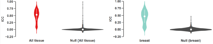
#导入包source("imp_functions.R")library(foreach)library(doParallel)library(psych)##plotViolin:使用ggplot2包生成小提琴图。plotViolin <- function(dfx, pltCol, ylim=NULL){ p <- ggplot(data=dfx, aes(x=type, y=ICC , fill=type,color=type)) p <- p + geom_boxplot(width = .001, outlier.size = 2.0, outlier.color = "#525252", outlier.shape = 95) p <- p + geom_violin(trim=F) p <- p + theme_classic() p <- p + scale_fill_manual(values=pltCol) p <- p + scale_color_manual(values=pltCol) p <- p + stat_summary(fun.data=data_summary, colour = "white", size=0.4) p <- p + theme(legend.position="none") p <- p + scale_y_continuous(breaks = seq(-1,1,by = 0.25)) p <- p + theme(axis.text.x = element_text(colour="grey20",size=12, angle=0,face="bold"), axis.text.y = element_text(colour="grey20",size=11, face="bold"), axis.title.y = element_text(colour="grey20",size=11, face="bold"), axis.ticks.length=unit(0.25,"cm")) p <- p + theme(axis.line.x = element_line(size = 0, colour = "white"), axis.title.x=element_blank(), axis.ticks.x=element_blank())if(!is.null(ylim)) { p <- p + coord_cartesian(ylim = ylim, expand = F) }return(p)}##computeRankMatFor1Gene函数:计算给定基因在样本中的排名矩阵 computeRankMatFor1Gene <- function(gn, pt, marExp){ findRankOfGene <- function(gn, sampleIds, marExp) { rtx <- rep(NA, length(sampleIds)); names(rtx)<- names(sampleIds)for(n in names(rtx)) {s <- sampleIds[n]if(!is.na(s)) { gval <- sort(marExp[, s]) rtx[n] <- which(names(gval)==gn) } }return(rtx) } gnRankMat <- matrix(data = NA, nrow = nrow(pt), ncol = ncol(pt)) rownames(gnRankMat) <- rownames(pt); colnames(gnRankMat)<- colnames(pt)for(patientID in rownames(pt)) { sampleIds <- pt[patientID, ] gnRankMat[patientID, ] <- findRankOfGene(gn, sampleIds, marExp) } gnRankMat <- gnRankMat[!apply(gnRankMat, 1, function(x)all(is.na(x))), ]return(gnRankMat)}##getICCforAllGen函数:用于计算所有基因的ICC(Intraclass Correlation Coefficient)。getICCforAllGenes <- function(pt, allGenes, marExp, NCPU=2, verbose=F){if(verbose==TRUE) { cl<-makeCluster(NCPU, outfile="") } else { cl<-makeCluster(NCPU)} registerDoParallel(cl) allICC <- foreach(i=1:length(allGenes), .export=c("computeRankMatFor1Gene"), .packages = c("psych") ) %dopar% { gn <- allGenes[i] gnRankMat <- computeRankMatFor1Gene(gn, pt, marExp) v <- NULLif(nrow(gnRankMat)>2) { v <- psych::ICC(gnRankMat, missing = F) v$geneName <- gn } v } stopCluster(cl) rtx <- data.frame()for(i in 1:length(allICC)) {if(!is.null(allICC[[i]])) { v <- allICC[[i]]$results["Single_raters_absolute",] v["gene"] <- allICC[[i]]$geneName rtx <- rbind(rtx, v[c("ICC", "p", "gene")]) } } rownames(rtx) <- NULLreturn(rtx) }## randomizeMatGetICC函数:用于对数据进行随机化处理,并计算随机化后的基因ICC值。randomizeMatGetICC <- function(passMatx, allGenes, marExp, NCPU, verbose=F){ passMatRand <- passMatxfor(i in 1:ncol(passMatRand)) { passMatRand[,i] <- sample(passMatRand[,i]) }for(i in 1:nrow(passMatRand)) { passMatRand[i,] <- sample(passMatRand[i,]) } passMatRand <- passMatRand[!(apply(passMatRand, 1, function(x) all(is.na(x)))),] rownames(passMatRand) <- paste0("r", 1:nrow(passMatRand)) allICCRand <- getICCforAllGenes(passMatRand, allGenes, marExp, NCPU=NCPU, verbose=verbose)return(allICCRand)}## 数据加载和准备NCPU = max(1, detectCores()-1 )cat(sprintf("n##---- number of CPU %d ------n", NCPU))passage <- readRDS("../data/passage_data.Rda")dp <- pData(passage$data)mar <- passage$dataallGenes <- rownames(mar)marExp <- Biobase::exprs(mar)pheno <- Biobase::pData(mar)pheno$passage <- paste0("P", pheno$passage)passMat <- passage$passageif(recompute==TRUE){ cat(sprintf("recomputing values.... it may take long timen")) ICCv <- list()##-------------------------------------------------------##------------------For all tissue type -----------------##------------------------------------------------------- allICC <- getICCforAllGenes(passMat, allGenes, marExp, NCPU=NCPU, verbose=F) allICC$type <- "All tissue" allICCRand <- randomizeMatGetICC(passMat, allGenes, marExp, NCPU=NCPU, verbose=F) allICCRand$type <- "Null (All tissue)" ICCv[["All tissue"]] <- rbind(allICC, allICCRand)##-------------------------------------------------------##------------------By Tissue Type ---------------------- tissueName <- c("breast", "lung", "pancreas", "skin", "large_intestine")for(tt in tissueName) { ptt <- passMat[pheno[pheno$tumor.type==tt, "patient.id"], , drop=F]if(nrow(ptt)>8) { cat(sprintf("##--- running for %s -----n", tt)) allICCtt <- getICCforAllGenes(ptt, allGenes, marExp, NCPU=NCPU, verbose=F) allICCtt$type <- tt allICCttRand <- randomizeMatGetICC(ptt,allGenes,marExp,NCPU=NCPU,verbose=F) allICCttRand$type <- sprintf("Null (%s)", tt) ICCv[[tt]] <- rbind(allICCtt, allICCttRand) }##储存结果 saveRDS(ICCv, "../results/ICC_for_genes.Rda") }} else {ICCv <- readRDS("../data/ICC_for_genes.Rda")}##绘制图片pltColo <- c('#e41a1c', '#8dd3c7','#bebada','#fb8072','#80b1d3','#fdb462')names(pltColo)<-c("All tissue","breast","lung","pancreas","skin","large_intestine")nullCol <- "#4d4d4d"pdf("../results/figure-3.pdf", width = 5.15, height = 2.15)for(tt in names(pltColo)){ dfx <- ICCv[[tt]] pltCol <- c(pltColo[tt], nullCol); names(pltCol) <- c(tt, sprintf("Null (%s)", tt)) dfx$type <- factor(as.character(dfx$type), levels = names(pltCol)) ylim <- c(-0.25,1) p <- plotViolin(dfx, pltCol, ylim = ylim)print(p)}dev.off()
 |
 |
小果还提供思路设计、定制生信分析、文献思路复现;有需要的小伙伴欢迎直接扫码咨询小果,竭诚为您的科研助力!
定制生信分析 服务器租赁 扫码咨询小果


|
01 |
|
02 |
|
03 |
|
04 |