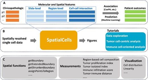
前言
谈起生信分析必备项目免疫浸润分析,小伙伴们再熟悉不过了!像小伙伴们耳熟能详的ImmuCellAL、Cibersort都只能在RNA-Seq和芯片数据中使用,像目前火爆的单细胞组学数据这两个R包却无用武之地!今天大海哥带大家学习如何在单细胞数据中进行免疫浸润分析!对,你没听错,单细胞中也可以进行免疫浸润分析。SpatialCells的功能涵盖了肿瘤微环境分析的各个方面,例如基于区域的细胞组成、肿瘤增殖指数、肿瘤分离指数、免疫细胞浸润和肿瘤免疫距离等。SpatialCells的功能实在太强大了,今天大海哥着重带大家学习单细胞中的免疫浸润分析!此外,SpatialCells 也有助于后续的关联分析和机器学习预测,使其成为推进我们对肿瘤生长、侵袭和转移理解的重要工具。生信分析不熟悉的小伙伴们欢迎来滴滴大海哥,大海哥就是这么的宠粉,有什么生信分析上的问题大家尽管咨询大海哥!没有时间学习的小伙伴们也不要着急哦!有需要生信分析的小伙伴们也可以找大海哥哦!练了十年生信分析的大海哥对于生信分析知识已经如鱼得水从分析到可视化直到你满意为止!
生信数据处理起来占用内存实在太大了,放过自己的电脑吧!大海哥在这里给大家送上福利了,有需要服务器的小伙伴们,欢迎大家联系大海哥,保证服务器的性价比最高哦!
代码教程
SpatialCells 目前只能从源安装。 要安装,请从存储库下载代码并切换到代码文件夹。
从 SpatialCells 的根目录运行以下命令:
pip install -r requirements.txt
pip install .
建议在虚拟环境中安装 SpatialCells,例如 conda。 可以使用以下 yaml 文件创建 conda 环境:
conda env create –name spatialcells –file=conda.yaml
pip install .
conda.yaml 指定如下:
name: spatial-cells-env
channels:
– conda-forge
– defaults
dependencies:
– python>=3.7, <3.11
– ipykernel
– matplotlib>=3.7.0
– pandas>=2.0.3
– seaborn>=0.12.2
– shapely>=2.0
– tqdm
– pip
– pip:
– anndata==0.9.2
– scanpy==1.9.4
加载相关的python包
import pandas as pd
import matplotlib.pyplot as plt
import anndata as ad
import spatialcells as spc
在本节中,我们以免疫细胞浸润分析为导向的分析的结果来展示 SpatialCells 的功能。我们的分析涉及由1110585个细胞组成的皮肤黑色素瘤样本(MEL1)的公开多路复用成数据。
读取和预处理数据
adata = ad.read_h5ad(“../../data/MEL1_adata.h5ad”)
spc.prep.setGate(adata, “KERATIN_cellRingMask”, 6.4, debug=True)
spc.prep.setGate(adata, “SOX10_cellRingMask”, 7.9, debug=True)
spc.prep.setGate(adata, “CD3D_cellRingMask”, 7, debug=True)
肿瘤边缘暴露于来自基质区域的细胞浸润、物理接触和可扩散趋化梯度,反之亦然。因此,定义肿瘤和基质边界使我们能够更具体地评估侵袭性黑色素瘤肿瘤细胞与微环境之间的复杂相互作用,并识别新的标记物。
分离肿瘤细胞群落并绘制区域边界
marker = [“SOX10_cellRingMask_positive”]
communitycolumn = “COI_community”
ret = spc.spatial.getCommunities(adata, marker, eps=60, newcolumn=communitycolumn)
fig, ax = plt.subplots(figsize=(10, 8))
spc.plt.plotCommunities(
adata, ret, communitycolumn, plot_first_n_clusters=10, s=2, fontsize=10, ax=ax
)
ax.invert_yaxis()
plt.show()

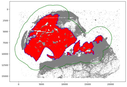
绘制肿瘤的区域边界
communityIndexList = [6, 3, 14, 51, 29, 47, 39, 44, 22]
boundary = spc.spatial.getBoundary(
adata, communitycolumn, communityIndexList, alpha=130
)
boundary = spc.spa.pruneSmallComponents(boundary, min_edges=50, holes_min_edges=500)
roi_boundary = spc.spa.getExtendedBoundary(boundary, offset=2000)
markersize = 1
fig, ax = plt.subplots(figsize=(10, 7))
## all points
ax.scatter(
*zip(*adata.obs[[“X_centroid”, “Y_centroid”]].to_numpy()),
s=markersize,
color=”grey”,
alpha=0.2
)
# Points in selected commnities
xy = adata.obs[adata.obs[communitycolumn].isin(communityIndexList)][
[“X_centroid”, “Y_centroid”]
].to_numpy()
ax.scatter(xy[:, 0], xy[:, 1], s=markersize, color=”r”)
# Bounds of points in selected commnities
spc.plt.plotBoundary(boundary, ax=ax, label=”Boundary”, color=”b”)
spc.plt.plotBoundary(roi_boundary, ax=ax, label=”ROI boundary”, color=”g”)
ax.invert_yaxis()
plt.show()
将细胞分配到肿瘤区域
spc.spatial.assignPointsToRegions(
adata,
[boundary, roi_boundary],
[“Tumor”, “Tumor_ROI”],
assigncolumn=”region”,
default=”BG”,
)
point_size = 1
fig, ax = plt.subplots(figsize=(10, 7))
for region in sorted(set(adata.obs[“region”])):
tmp = adata.obs[adata.obs.region == region]
ax.scatter(
*zip(*tmp[[“X_centroid”, “Y_centroid”]].to_numpy()),
s=point_size,
alpha=0.7,
label=region
)
# Bounds of points in selected commnities
spc.plt.plotBoundary(boundary, ax=ax, label=”Boundary”, color=”purple”)
spc.plt.plotBoundary(roi_boundary, ax=ax, label=”ROI boundary”, color=”r”)
plt.legend(loc=”upper right”)
ax.invert_yaxis()
plt.show()

根据现有表型概括细胞类型
def merge_pheno(row):
if row[“phenotype_large_cohort”] in [
“T cells”,
“Cytotoxic T cells”,
“Exhausted T cells”,
]:
return “T cells”
elif row[“phenotype_large_cohort”] in [“Melanocytes”]:
return “Tumor cells”
else:
return “Other cells”
def cell_type(row):
if row[“SOX10_cellRingMask_positive”]:
return “SOX10+”
elif row[“CD3D_cellRingMask_positive”]:
return “CD3D+”
else:
return “Other cells”
# Applying the function to create the new columns
adata.obs[“pheno1”] = pd.Categorical(adata.obs.apply(merge_pheno, axis=1))
adata.obs[“Cell Types”] = pd.Categorical(adata.obs.apply(cell_type, axis=1))
spc.msmt.getRegionComposition(adata, “pheno1”)
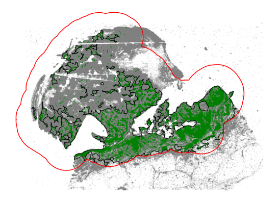
在肿瘤ROI区域找到免疫细胞浸润区域
melano = adata[
(adata.obs.SOX10_cellRingMask_positive) & (adata.obs.region.isin([“Tumor_ROI”, “Tumor”]))
]
tcells = adata[
(adata.obs.CD3D_cellRingMask_positive)
& (adata.obs.region.isin([“Tumor_ROI”, “Tumor”]))
]
fig, ax = plt.subplots(figsize=(10, 7))
ax.invert_yaxis()
ax.set_aspect(“equal”)
plt.scatter(
tcells.obs[“X_centroid”],
tcells.obs[“Y_centroid”],
s=0.5,
label=”T cells”,
color=”green”,
alpha=0.5,
)
spc.plt.plotBoundary(roi_boundary, ax=ax, label=”ROI boundary”, color=”r”)
plt.legend(loc=”upper right”, markerscale=5)
plt.show()

tumor = adata[adata.obs.region.isin([“Tumor_ROI”, “Tumor”])]
communitycolumn = “CD3D_cellRingMask_positive”
communityIndexList = [True]
immune_boundary = spc.spatial.getBoundary(
tumor, communitycolumn, communityIndexList, alpha=130
)
immune_boundary = spc.spa.pruneSmallComponents(
immune_boundary, min_edges=25, holes_min_edges=30, min_area=30000
)
markersize = 0.1
fig, ax = plt.subplots(figsize=(10, 7))
## all points
ax.scatter(
*zip(*adata.obs[[“X_centroid”, “Y_centroid”]].to_numpy()),
s=markersize,
color=”grey”,
alpha=0.2
)
# Points in selected commnities
xy = tumor.obs[tumor.obs[communitycolumn].isin(communityIndexList)][
[“X_centroid”, “Y_centroid”]
].to_numpy()
ax.scatter(xy[:, 0], xy[:, 1], s=markersize, color=”green”, alpha=1, label=”T cells”)
# Bounds of points in selected commnities
spc.plt.plotBoundary(
immune_boundary, ax=ax, label=”Immune Cell Region Boundary”, color=”k”, linewidth=1
)
spc.plt.plotBoundary(roi_boundary, ax=ax, label=”ROI boundary”, color=”r”)
# ax.set_xlim(0, 20000)
# ax.set_ylim(0, 13000)
ax.invert_yaxis()
ax.set_aspect(“equal”)
ax.set_axis_off()
# plt.legend(loc=”upper right”, markerscale=5, fontsize=13.5)
# plt.savefig(“immune_cell_region1.png”, dpi=400)
plt.show()
spc.spatial.assignPointsToRegions(
melano, [immune_boundary], [“T”], assigncolumn=”tumor_isolated_region”, default=”F”
)
我们可以通过将已识别的免疫浸润区域与所有肿瘤细胞重叠来估计免疫浸润的规模。
point_size = 0.5
fig, ax = plt.subplots(figsize=(10, 7))
ax.scatter(
*zip(*adata.obs[[“X_centroid”, “Y_centroid”]].to_numpy()),
s=markersize,
color=”grey”,
alpha=0.2
)
colors = [“red”, “orange”]
labels = [“Immune-isolated Tumor Cells”, “Immune-rich Tumor Cells”]
for i, region in enumerate(sorted(set(melano.obs[“tumor_isolated_region”]))):
tmp = melano.obs[melano.obs.tumor_isolated_region == region]
ax.scatter(
*zip(*tmp[[“X_centroid”, “Y_centroid”]].to_numpy()),
s=point_size,
alpha=0.5,
color=colors[i],
label=labels[i]
)
# Bounds of points in selected commnities
spc.plt.plotBoundary(
immune_boundary, ax=ax, label=”Immune Cell Region Boundary”, color=”k”, linewidth=1
)
spc.plt.plotBoundary(roi_boundary, ax=ax, label=”ROI boundary”, color=”b”)
ax.invert_yaxis()
ax.set_axis_off()
# plt.savefig(“roi_region1.png”, dpi=400)
plt.show()

print(“Percentage of tumor cells in immune-isolated regions: “)
melano.obs[“tumor_isolated_region”].value_counts() / len(melano.obs)
我们还可以通过比较肿瘤区域和免疫细胞区域之间的区域重叠来观察免疫浸润的规模。
roi_area = spc.msmt.getRegionArea(roi_boundary)
tumor_area = spc.msmt.getRegionArea(boundary)
immune_area = spc.msmt.getRegionArea(immune_boundary)
tumor_immune_overlap = boundary.intersection(immune_boundary)
overlap_area = spc.msmt.getRegionArea(tumor_immune_overlap)
print(f”Area of ROI: {roi_area:.2f}”)
print(f”Area of main tumor cell region: {tumor_area:.2f}”)
print(f”Area of immune cell region: {immune_area}”)
print(f”Area of overlap between tumor and immune cell regions: {overlap_area:.2f}”)
print(
f”Percentage of tumor region that has overlap with “
f”immune cell region: {overlap_area / tumor_area:.3f}”
)
识别与免疫细胞相邻的肿瘤细胞。
dists = spc.msmt.getMinCellTypesDistance(melano, tcells)
adata.obs.loc[
(adata.obs.SOX10_cellRingMask_positive) & (adata.obs.region.isin([“Tumor_ROI”, “Tumor”])), “dist”
] = dists
threshold = 20
adata.obs[“dist_binned”] = adata.obs[“dist”] <= threshold
infiltrated = adata.obs[
(adata.obs.SOX10_cellRingMask_positive)
& (adata.obs.region == “Tumor”)
& (adata.obs.dist_binned == True)
]
non_infiltrated = adata.obs[
(adata.obs.SOX10_cellRingMask_positive)
& (adata.obs.region == “Tumor”)
& (adata.obs.dist_binned == False)
]
fig, ax = plt.subplots(figsize=(10, 6))
ax.invert_yaxis()
region = adata.obs[(adata.obs.region == “Tumor”)]
plt.scatter(region[“X_centroid”], region[“Y_centroid”], s=1, alpha=0.2, color=”grey”)
plt.scatter(
infiltrated[“X_centroid”],
infiltrated[“Y_centroid”],
s=1,
alpha=0.5,
color=”green”,
label=f”Infiltrated (distance to t-cells <= {threshold}um)”,
)
plt.legend(markerscale=10)
plt.show()

小结
SpatialCells 是一个用于空间分析多路复用单细胞成像数据的软件包,其特点是能够根据任何细胞组定义感兴趣区域,然后进行基于区域的分析。SpatialCells的功能涵盖了肿瘤微环境分析的各个方面,例如基于区域的细胞组成、肿瘤增殖指数、肿瘤分离指数、免疫细胞浸润和肿瘤免疫距离。SpatialCells 允许使用用户定义的参数以标准化方式预处理和分析数据,并且可以处理包含数百万个细胞的样本。最后大海哥给大家介绍一个云工具!同学们如果觉得自己的代码水平一般,对于很多的参数不知道怎么改,可以体验一下我们的云生信小工具,只需输入数据,即可轻松生成所需图表,字体大小、标题等也可一键更改。感兴趣的小伙伴去云生信(http://www.biocloudservice.com/home.html)体验一下吧!